Figures and data in Patterning precision under non-linear morphogen decay and molecular noise | eLife

Figures
Additional files

6 figures and 1 additional file

Figures

Figure 1

Download asset Open asset

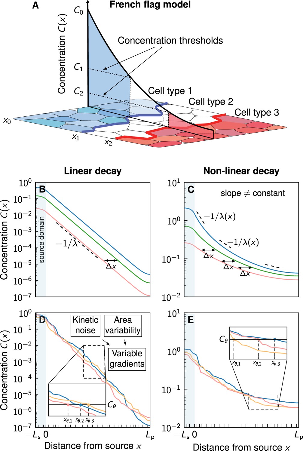
Comparison of linear and non-linear morphogen gradients.

(A) According to the French flag model, morphogen gradients provide the spatial information required for tissue patterning via concentration thresholds $C_{θ}$ , numbered by $θ = 1, 2, 3$ etc. If a cell lies above or below a certain threshold $C_{θ}$ , it switches fate, resulting in domain boundaries forming at the respective cell borders at $x = x_{θ}$ (blue and red lines). The morphogen source is located at $x = x_{0} = 0$ . (B) Linear decay leads to exponential gradients. Changes in the gradient amplitude C₀ (different colours) lead to a shift $Δ x$ that is independent of the amplitude. (C) Non-linear decay ( $n = 2$ ) leads to power-law gradients. The shift $Δ x$ due to a change of C₀ is amplitude-dependent. (D, E) Noisy example gradients obtained numerically. Cell boundaries are denoted by black ticks along the patterning axis. Molecular kinetic noise and cell area variability leads to noisy gradients. For a fixed readout threshold $C_{θ}$ , variable gradients result in different readout positions $x_{θ, j}$ (inset plots). Non-linear decay (E) leads to shallower gradients further in the patterning domain compared to linear decay (D).

Figure 2

Download asset Open asset

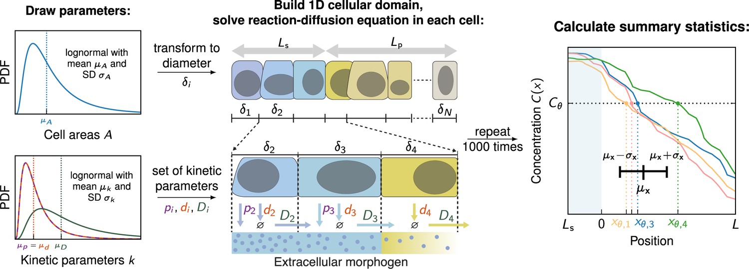
Numerical model to simulate noisy gradients.

A 1D cellular domain is constructed by drawing cell areas from log-normal distributions with mean cell area $μ_{A}$ and standard deviation $σ_{A}$ . Cell areas are then converted to diameters ( $δ_{i}$ ). This procedure is repeated $N$ times until source and patterning domains of length $L_{s}$ and $L_{p}$ are filled with cells. Kinetic parameters $k = p, d, D$ are drawn independently from log-normal distributions with a mean $μ_{k}$ and standard deviation $σ_{k}$ for each cell. Production only takes place in the source (blue cells). Then, the reaction-diffusion equation (Equation 6) is solved on the cellular domain, generating one noisy gradient $C_{j} (x)$ . To determine a unique readout concentration of a cell, the average concentration along the cell boundary is computed for each cell in the patterning domain. Based on these concentrations the readout position $x_{θ, j}$ where $C_{j} (x_{θ, j}) = C_{θ}$ is recorded for each gradient. This step is repeated 1000 times. Lastly, the average readout position $μ_{x}$ and the positional error $σ_{x}$ is calculated based on the 1000 noisy gradients. PDF denotes the probability density function.

Figure 3

Download asset Open asset

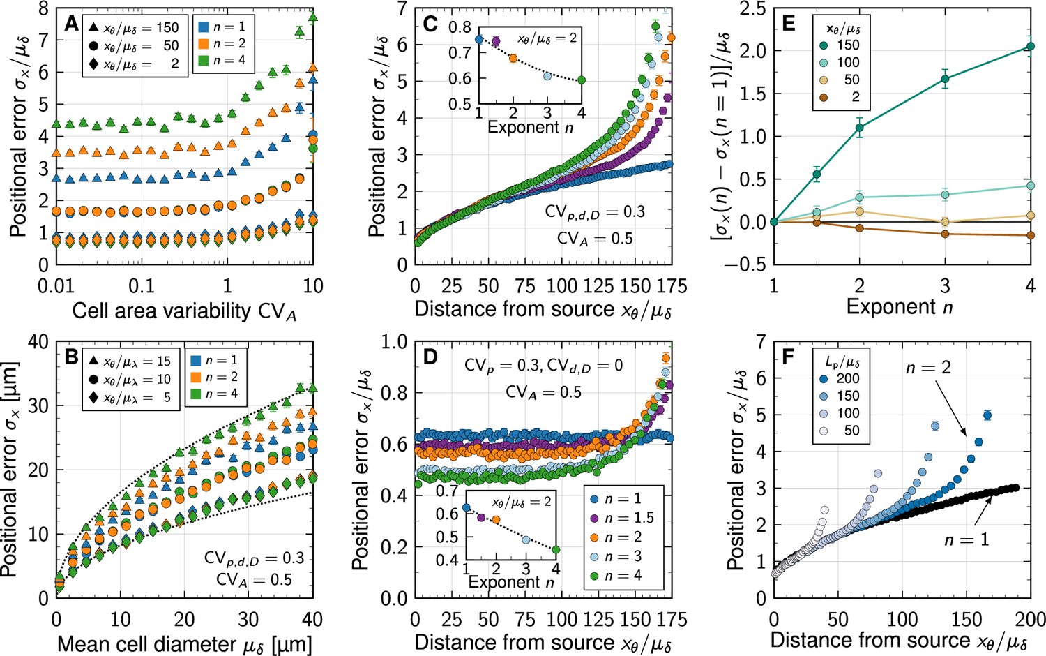
Impact of non-linear decay on gradient precision.

(A) Physiological variability in the cross-sectional cell areas has no significant impact on gradient precision. The positional error $σ_{x}$ is plotted in units of the mean cell diameter $μ_{δ}$ at different readout positions in the patterning domain (symbols), and for different degrees of non-linearity (colours). (B) The positional error increases with the square root of the cell diameter, irrespective of $n$ . Dotted lines show $σ_{x} = α \sqrt{μ_{δ}}$ for $α = 2.6, 5.2$ for reference, with lengths in units of µm. $L_{p} = 100 μ_{δ}$ . (C) Non-linear decay leads to a marginally lower positional error close to the morphogen source. Inset plot shows $σ_{x} / μ_{δ}$ at a distance of two cells from the source as a function of decay non-linearity. With a no-flux boundary at $x = L_{p}$ , the shallowness of gradients from non-linear decay lets the positional error increase strongly far from the source. Colours correspond to different decay exponents $n$ , as specified in panel D. (D) Variability in the production rate alone has no effect on the positional error along the domain for linear decay (blue). The stronger the non-linearity, the smaller the positional error close to the source (inset). Far from the source, the positional error increases rapidly with non-linear decay. (E) Difference between the positional error for $n > 1$ and for $n = 1$ relative to the mean cell diameter, at fixed readout positions (colours). (F) Effect of finite patterning domain size. The positional error increases close to the distant zero-flux boundary in case of non-linear decay (shades of blue, $n = 2$ ). Patterning remains precise across a larger distance in the case of linear decay (black, $n = 1$ ). In all panels, each data point represents the mean from 10³ independent simulations. Error bars represent standard errors.

Figure 4

Download asset Open asset

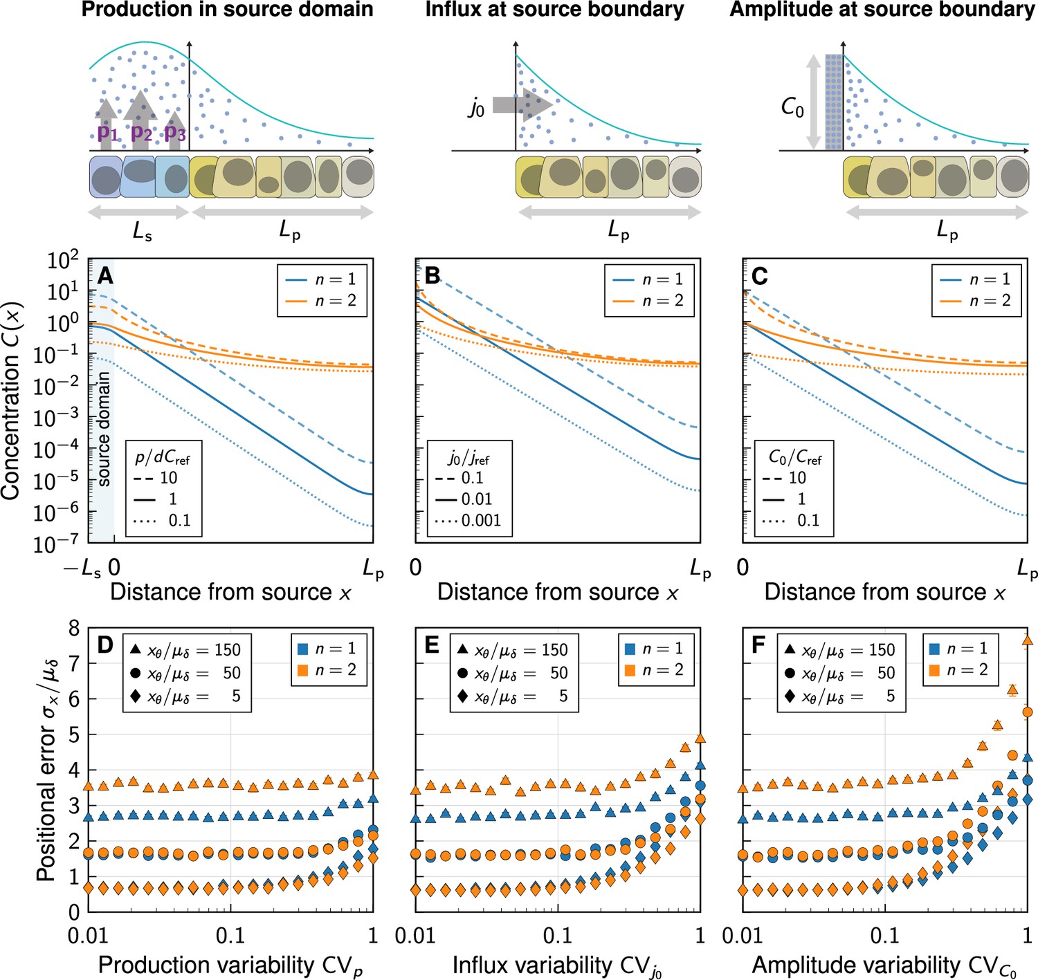
Impact of the boundary condition (BC) at the source.

(A–C) Noise-free gradient shapes when the morphogen is either secreted in a source domain at rate $p$ (Equation 6) (A), with flux BC, $- {D \partial C / \partial x |}_{x = 0} = j_{0}$ (B), or Dirichlet BC, $C (0) = C_{0}$ (C). No-flux BC were imposed at at the far end of the tissue (at $x = L_{p}$ ). (D–F) Positional error as a function of morphogen abundance variability, at different readout positions (symbols) and degrees of non-linearity (colours). Greater variability in the morphogen production rate (D), influx (E), and gradient amplitude (F) leads to a larger positional error above a certain threshold variability $C V ⪆ 0.1 - 0.3$ . Kinetic variability was fixed at ${C V}_{d, D} = 0.3$ (except for ${CV}_{p}$ in D). Further parameters: $μ_{j_{0}} = μ_{D} C_{ref} / μ_{λ}$ (E), $μ_{C_{0}} = C_{ref}$ (F). In panels D–F, each data point represents the mean from 10³ independent simulations. Error bars represent standard errors.

Figure 5

Download asset Open asset

Impact of the morphogen source strength.

Numerically obtained spatial patterning accuracy in units of average cell diameters $μ_{δ}$ at different positions in the tissue (symbols) and for different degrees of non-linearity (colours). (A–C) Readout close to the source, at $x_{θ} = 5 μ_{δ}$ ; (D–F) Readout far from the source, at $x_{θ} = 150 μ_{δ}$ . Morphogen production scenarios are identical to Figure 4: Production in a source domain with morphogen-secreting cells (A,D), with a morphogen influx from the source at the source boundary (B,E), and with a specified morphogen concentration at the source boundary (C,F). Very low (high) influxes or amplitudes lead to flat (steep) gradients at strong decay non-linearity, limiting the parameter range over which the positional error can be reliably determined for $n = 4$ (B,C,E,F). In all panels, each data point represents the mean from 10³ independent simulations, error bars represent standard errors.

Appendix 1—figure 1

Download asset Open asset

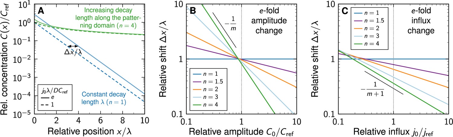
Shift in morphogen gradients due to changes in morphogen production.

(A) Comparison of noise-free gradients arising from linear (blue) and non-linear (green) decay. A fold-change in the influx j₀ from the source shifts the gradients by $Δ x$ . (B) Positional shift of the morphogen gradient as a function of the amplitude and degree of non-linearity, for a fold-change in the amplitude, $C_{0}^{*} / C_{0} = e$ . (C) Positional shift as a function of the influx and degree of non-linearity, for a fold-change in the influx, $j_{0}^{*} / j_{0} = e$ .

Additional files

MDAR checklist: https://cdn.elifesciences.org/articles/84757/elife-84757-mdarchecklist1-v1.pdf
Download elife-84757-mdarchecklist1-v1.pdf

Download links

A two-part list of links to download the article, or parts of the article, in various formats.

Downloads (link to download the article as PDF)

Article PDF

Open citations (links to open the citations from this article in various online reference manager services)

Mendeley

Cite this article (links to download the citations from this article in formats compatible with various reference manager tools)

Jan Andreas Adelmann
Roman Vetter
Dagmar Iber

(2023)

Patterning precision under non-linear morphogen decay and molecular noise

eLife 12:e84757.

https://doi.org/10.7554/eLife.84757

Sign up for email alerts

Privacy notice