Structure of the HIV immature lattice allows for essential lattice remodeling within budded virions
- TC Jenkins Department of Biophysics, Johns Hopkins University, United States
- Laboratory of Cell and Developmental Signaling, Center for Cancer Research, National Cancer Institute, National Institutes of Health, United States
- Center for Cell and Genome Science, University of Utah, United States
- Department of Physics and Astronomy, University of Utah, United States
- School of Biological Sciences, University of Utah, United States
Figures
Figure 1 with 4 supplements
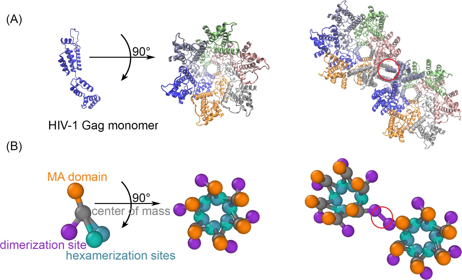
The structure-resolved reaction-diffusion model for Gag assembly on spherical membranes.
(A) The Gag monomers from the cryoET structure of the immature lattice (Schur et al., 2016) taken from 5L93.pdb is shown on its own, as part of a single hexamer (center), and with a dimerization interface in the red circle that brings together two hexamers (right). (B) Our coarse-grained model is derived from this structure to place interfaces on each monomer at the position where they bind. The reaction network contains three types of interactions. The MA domain (orange) binds to the membrane. The position of the MA site is not in the cryoET structure, and we position it to place each monomer normal to the surface. The distance of the MA site from the center of mass is set to 2 nm. The hexamerization sites (green and blue) mediate the front-to-back binding between monomers to form a cycle. The dimerization site (purple) forms a homo-dimer between two Gag monomers, as illustrated on the right. The reactive sites are point particles that exclude volume only with their reactive partners at the distances shown. Thus, the hexamer-hexamer binding radius is 0.42 nm, whereas the longer dimer-dimer binding radius is 2.21 nm. Positions and orientations are defined in Source Data. The experimental lattice has an intrinsic curvature, and our model recapitulates this to assemble a sphere. The binding kinetics between the interaction types for multiple rates was validated against theory (Figure 1—figure supplements 1 and 2), and we verified that the lipid binding site model did not significantly impact the dynamics of the lattice (Figure 1—figure supplement 3). The positioning of the Gag interfaces in this model of the immature lattice are distinct from a model that would assemble the mature lattice (Figure 1—figure supplement 4).
-
Figure 1—source data 1
Model Coordinates.
Binding site positions, binding radius, and binding angles of the coarse model in Figure 1.
- https://cdn.elifesciences.org/articles/84881/elife-84881-fig1-data1-v2.xlsx
Figure 1—figure supplement 1
Kinetics of dimer formation between Gag monomers is consistent with theory.
In these simulations, only the homo-dimer contacts could form, and the hexamer sites were turned off. Thus, the kinetics of reversible dimerization from NERDSS simulations (colored lines) can be compared with the non-spatial rate-equation solution (black dashed). Here, we initialized all monomers to be on the membrane surface irreversibly, so the binding is purely in 2D. For each model, 5–10 trajectories were collected and averaged. As the microscopic association rate ka was increased, we also increased the dissociation rate kb the same amount, so that the free energy was fixed for all simulations at –11.9kBT. The apparent 3D rates for the slowest system were ka3D=0.025 nm3/μs and kb = 0.1 s–1. The length-scale to convert from 3D rates to 2D rates was set here to h=5 nm, hence the slowest 2D rate is ka2D=0.005 nm2/μs. Initial copy numbers were 66 on the same membrane sphere with R=67 nm. D=0.2 nm2/μs and σ=2.21 nm. For the analytical solution in black dashed, we input the corresponding macroscopic 2D rates kon2D and koff2D. The macroscopic on-rate kon2D≤ ka2D due to its dependence on diffusion constants and the system size. We note that the agreement is not perfect between the reaction-diffusion simulations and the non-spatial solution. Although the kinetics are not expected to be identical in 2D due to sensitivity to spatial fluctuations, there is some disagreement because in the RD simulations, some of the association events were rejected if the monomers were not aligned closely enough to their target bound state, which causes a relative slow-down in the association rates. Specifically, we found that the rates that we assigned via the input files, for instance ka2D=0.02 nm2/μs, when simulated, produced kinetics with an apparent rate that was 4× slower. This same factor of 4 slow-down was observed for input rates of 0.2 and 2 nm2/μs. The dissociation kinetics are unaffected. We reject association events that cause a reorientation of the monomers into the bound state that is larger than our specified threshold. Our threshold is controlled by a scale-factor (scaleMaxDisplace) that was set low enough (to 10) for the slowly diffusing and non-rotating 2D monomers that events were rejected. We therefore report throughout the paper the rates that describe the actual observed kinetics and are thus 4× lower than the values we specified in our input files. We performed the same validation for the Gag monomers to form hexamers, with the dimer interaction turned off but still excluding volume. Here, again we found the same 4× slow-down in association kinetics relative to the assigned rates in the input file. Therefore, we always report these apparent rates that accurately describe the kinetics.
Figure 1—figure supplement 2
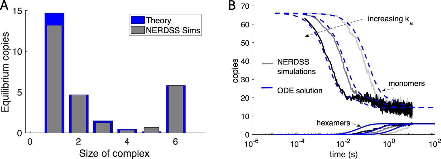
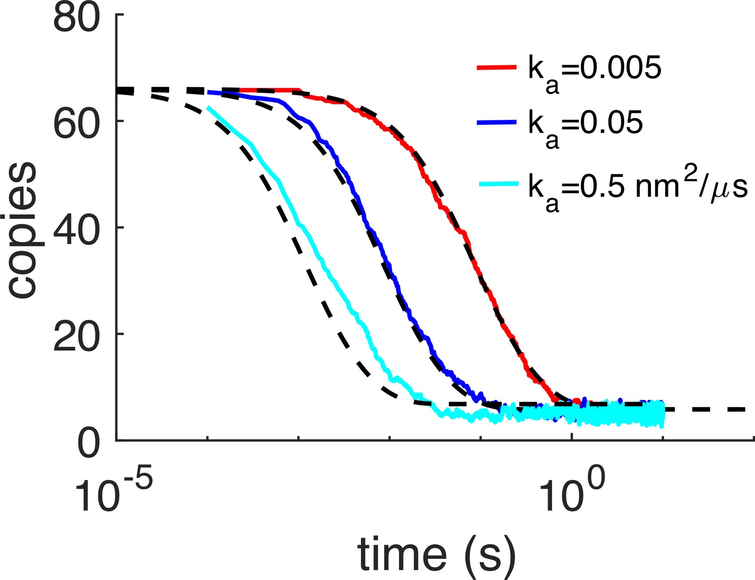
NERDSS simulations of purely hexamer assembly in 2D are validated against theory.
(A) Here, the Gag monomers could only bind through their hexamer sites, and the dimer sites were turned off (but could still exclude volume). With 66 initial Gag monomer copies initialized irreversibly on the spherical surface, the monomers could assemble into complexes from dimers up through to completed hexamers purely in 2D. The equilibrium yield here calculated numerically (blue bars) which agrees very well with the simulated equilibrium (gray bars). The free energy is ∆Ghex = −8.93kBT. When the hexamer loop closes, the strength of the final two bonds is slightly less than 2∆Ghex, and instead is 2∆Ghex+2.3kBT. We introduce this small penalty to mimic that the hexamer structure is not ideal. (B) We compare the kinetics of assembly from the NERDSS simulations (gray solid lines) with a set of non-spatial ordinary differential equations (ODEs) for hexamer formation solved numerically in MATLAB. The monomer population decreases from 66 copies (upper curves), while the hexamers assemble to their equilibrium value of ~6 (lower curves). The free energy for all simulations is the same as described in (A), and the microscopic rates increase from right to left as ka3D=0.025, 0.25, and 2.5 nm3/μs, with the length-scale from 3D to 2D set at the same value used in the full system as h=10 nm. The microscopic dissociation rates thus also increase accordingly from 2 to 200 s–1. Diffusion D=0.2 nm2/μs for each membrane-bound monomer, and the binding radius for the hexamer interaction is σ=0.418 nm The agreement between the NERDSS simulations and the ODEs are relatively strong, although the simulated hexamers assemble more slowly. This is in large part due to the excluded volume of the monomers (via their dimer sites) that slows the collisions between the reactive hexamer sites.
Figure 1—figure supplement 3

Comparison of the dynamics of remodeling simulations using the implicit lipid model and explicit lipids.
(A) Time dependence of the size of the largest assembled complex during the simulation. (B) Time dependence of the number of fragments in the system. A fragment is a complex with at least 30 Gags. and ka2D (nm2/μs)=2.5 × 10–2 for both implicit and explicit simulations. Overall the agreement is very close, with small deviations between the equilibrated number of fragments for this unstable system, likely due to the assumption in the implicit lipid model that the lipids are well mixed, which could speed up rebinding times. The proteins still remain affixed to the 2D membrane surface with explicit or implicit lipid sites.
Figure 1—figure supplement 4
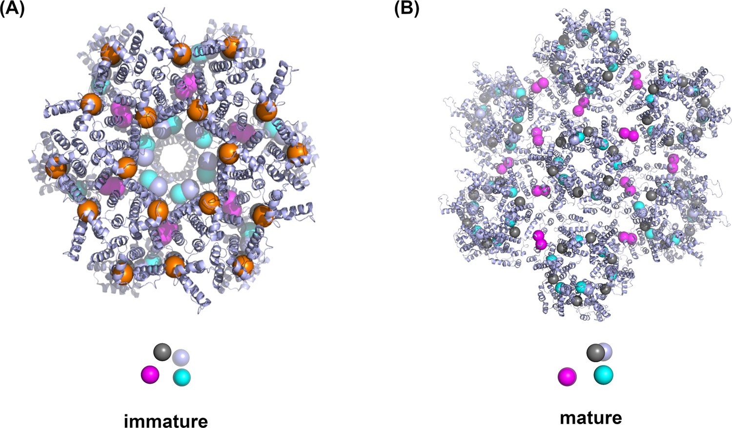
Comparison of the coarse-grained model of Gag monomer from the immature and mature lattice.
(A) The cartoon representation shows the experimental HIV-1 immature lattice structure from 5L93.pdb with 18 Gag monomers. To determine the position of the interaction sites between adjacent Gag monomers for the coarse-grained model, we calculated the average positions of all the atoms within a cutoff distance 0.35 nm from adjacent Gag monomers. The resulting interaction sites are represented with beads. Gray beads are the centers-of-mass (COM) of one Gag monomer. Cyan and light blue beads indicate the hexamerization sites, and magenta beads show the homo-dimerization sites between hexamers. The orange beads are the membrane binding sites, which are not included in the experimental structure but placed manually 2 nm above the COM in the direction normal to the membrane surface. A coarse-grained Gag monomer is depicted below the 18 Gag monomers complex. (B) The experimental HIV-1 mature capsid structure (3J34.pdb) and the coarse-grained model derived using the same method as in the determination of model for the immature lattice. A coarse-grained Gag monomer is illustrated below the 42 Gag monomers complex for the mature lattice system.
Figure 2 with 1 supplement
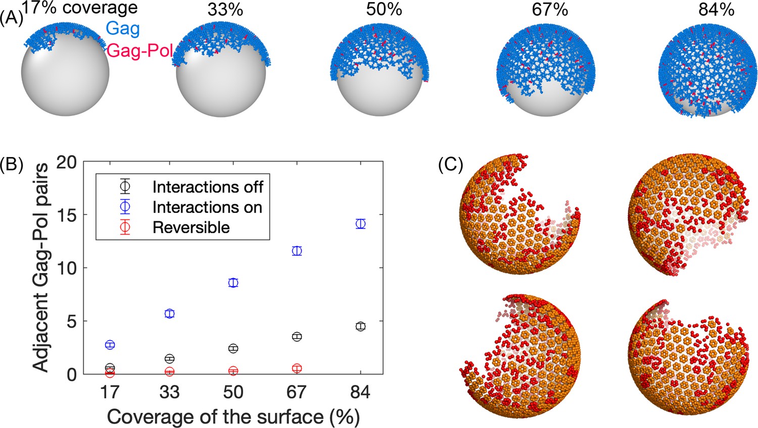
Initial Gag immature lattices within the membrane are assembled via simulation.
(A) The starting Gag immature lattices are assembled from NERDSS simulations with irreversible binding; ~5% of the monomers are Gag-Pols shown in red. We note that the silver spheres are shown here only to improve visualization of just one side of the lattice; Gag proteins are attached to the inner surface of the budded spherical membrane, consistent with experiment. (B) The number of adjacent pairs of Gag-Pol in the initial immature lattice increases with more surface coverage. Normally, we set all parameters for Gag and Gag-Pol to be identical (blue circles). During assembly, we tested turning off any explicit Gag-Pol to Gag-Pol interactions, rendering them unfavorable (black circles), but they can still end up adjacent to one another. However, this is sensitive to the assembly conditions—when monomers can unbind during assembly, they can correct these unfavorable interactions and reduce the Gag-Pol to Gag-Pol pairs further (red circles). (C) Formation of the lattice produces structures that are similar to cryoET, with a single large continent and a large vacancy, as well as several defects or incomplete hexamers throughout the large lattice, which are shown in red in these four independent assemblies. An incomplete hexamer in the simulated lattice is quantified as a sub-structure with 2–5 monomers present in the ring. The size distribution of these defect regions is also found to be similar to the cryoET results (Figure 2—figure supplement 1).
Figure 2—figure supplement 1
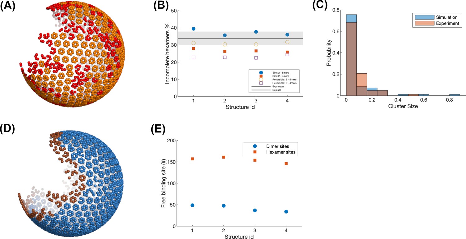
Quantitative analysis of the defects in the structures of our model and cryoET.
(A) Incomplete (red) and complete (orange) hexamers in the assembled lattice using our model. Each bead represents the center-of-mass (COM) of one Gag. Isolated monomers are also colored in red. (B) Comparison of the density of incomplete hexamers between our simulation and the experimental analysis. Experimental data is kindly provided by Prof. John Briggs. Experimental counts of incomplete hexamers had 3–5 monomers, as lower density was not reliably assigned a hexamer structure. The gray line represents the experimental value statistic from six viruses. Total hexamers in experimental lattices varied from ~300 to 530. Blue points are the simulation values for four different structures from our model, where the incomplete hexamer includes 2–5 monomers. Red points are the simulation values where the incomplete hexamer is the one that includes 2–4 monomers. Total hexamers in simulated lattices across four structures did not vary significantly as they all had very similar monomer numbers, from 550 to 565 total hexamers, similar to the most densely coated experimental lattice. The open symbols show the same statistics from simulations where the assembly allowed for unbinding of monomers (koff = 100 s–1 and 14 s–1 for hexamer and dimer), which reduced the total number of incomplete hexamers. (C) The comparison of the cluster size of incomplete hexamers distribution between the simulation and experiment. Two incomplete hexamers whose COM are within the cutoff distance of 1.2 * d are considered to belong to the same cluster, where d is the regular distance between two adjacent complete hexamers. The x-axis value is normalized to the total number of incomplete hexamers in one structure, thus 0.8 indicates 80% of incomplete hexamers are in one strand, which has low probability. (D) Edge hexamers (brown) in the same lattice as shown in (A). The Gag having less than 39 Gags within the distance 15 nm is considered as an edge Gag. The hexamers including edge gags are edge hexamers. (E) The number of available free hexamer binding sites (red points) and dimer binding sites (blue points) within the edge hexamers.
Figure 3 with 2 supplements
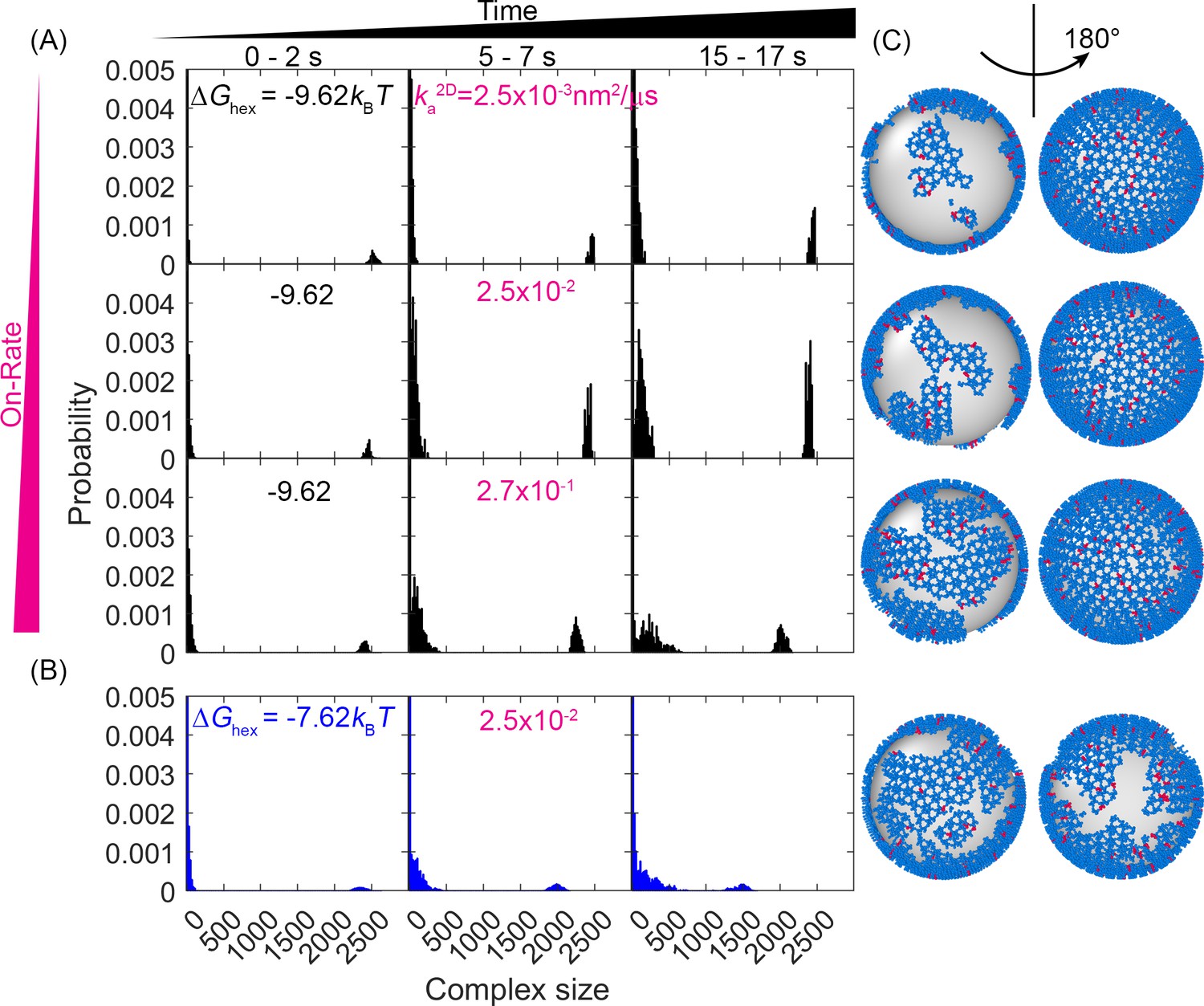
Evolution of the lattice size distribution at different reaction rates and hexamer interaction strengths.
(A) Along the x-axis are the numbers of monomers found in each lattice, which is largely bimodal for all systems: a population of small oligomers and one giant connected component. As time progresses (from left to right columns), the initial structure which was one giant connected component continues to fragment somewhat, indicating that the starting structure was not at equilibrium. As the on- and off-rates increase (from top to bottom) with a fixed , the largest component shrinks, as shown by the peak denoting the large giant component shifting to the left, and the peak denoting the small oligomers shifting to the right. (B) For a weaker hexamer free energy shown in the blue data (), the lattice is breaking apart more rapidly and moving toward a more uniform distribution of lattice patch sizes as both peaks shift to the center. Note that we cut off the y-axis at 0.005 to make the peak at ~2500 visible. The bars at small sizes extend up to ~0.05. (C) Representative structures at the later times (t=17 s) for each case, illustrating the increased fragmentation as the rates accelerate, or as the hexamer contacts destabilize (lowest row). We quantify the corresponding diffusivity of the structures in Figure 3—figure supplement 1. We show how changes to have a minimal impact on the structural dynamics in Figure 3—figure supplement 2.
Figure 3—figure supplement 1

Distribution of the diffusion constant of each molecule.
The right-most bar reports diffusion of monomers. The left-most bars are the molecules within the largest complex. A clear separation of timescales emerges as the lattice stabilizes due to the giant connected component. The rate constant for these simulations was the intermediate value of 0.025 nm2/µs.
Figure 3—figure supplement 2
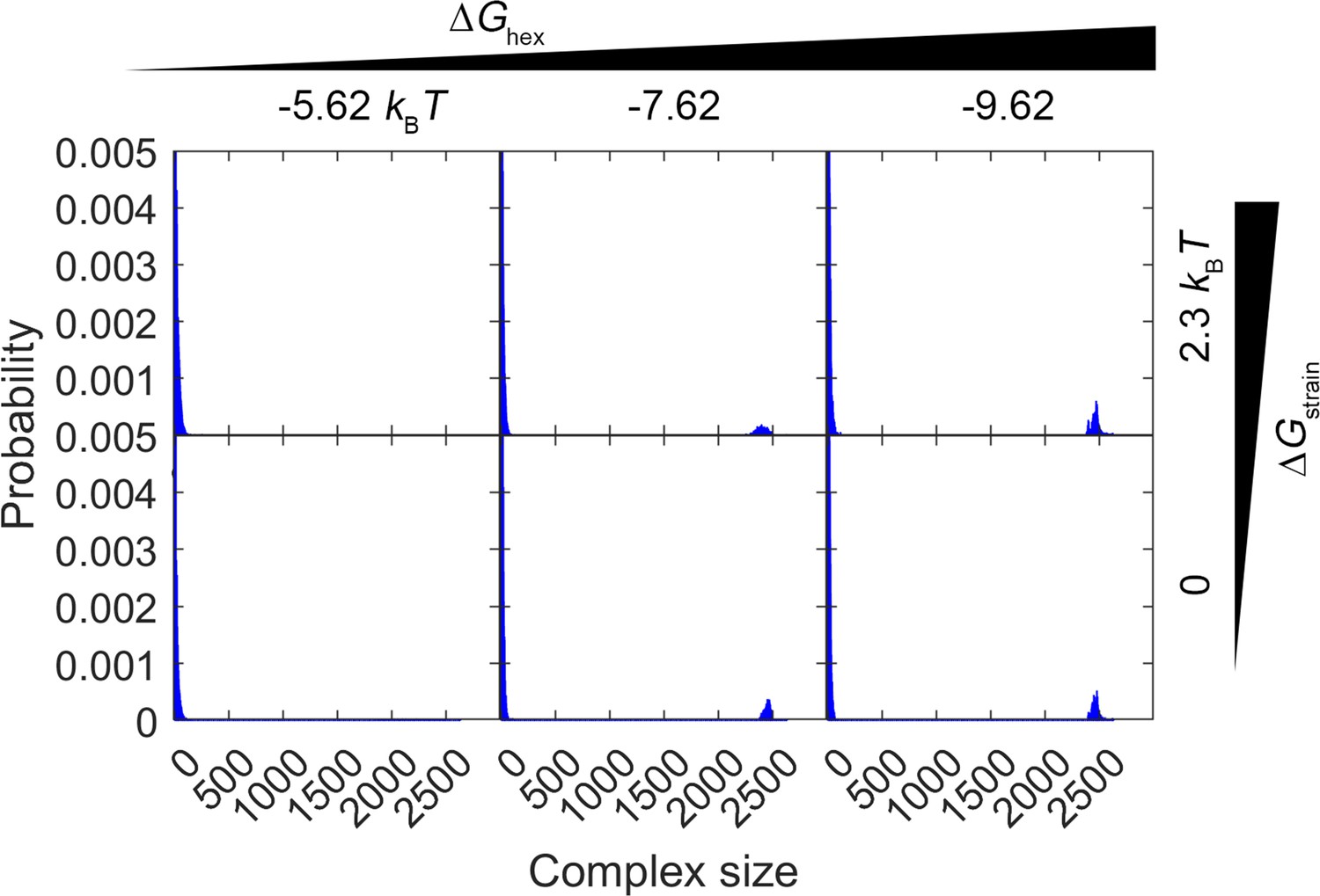
Comparison of complex size distribution over the first 0–1 s of simulations with two values of .
The top row shows the results for , the same value used in Figure 3 and all other simulations. Each column is a different value of . In the bottom row, we remove the strain penalty, , and therefore the closed hexamers have a 10-fold longer lifetime. The distributions are very similar in both cases, as the lattice stability is dominated by the value of . With the more stable lattices in particular () the closed hexamers have long lifetimes in both cases of strain (>25 s) and the dynamics is controlled by the partial incomplete hexamer structures on the edge.
Figure 4 with 1 supplement
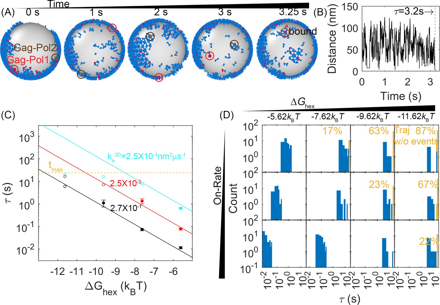
First-passage times (FPTs) for a pair of Gag-Pol monomers to search and bind to one another reveal a clear dependence on hexamer rates and free energies.
(A) An example from a simulation of how two Gag-Pols found each other. Characterization of the edge connectivity in Figure 4—figure supplement 1. (B) The distance between all Gag-Pol pairs can be monitored in time, with this trace corresponding to the simulation in (A). The distance fluctuates and drops to the binding radius σ at 3.2 s, after which the two molecules remain bound. (C) FPTs of Gag-Pol dimerization at different reaction rates and hexamer free energies . The yellow dashed line indicates the maximal length of the simulation traces. The filled-in circles report the mean FPT (MFPT) for parameter sets where all traces produce a Gag-Pol dimerization event. The open circles report a lower bound on the MFPT, because some of the traces were not long enough to observe a Gag-Pol dimerization event. The solid lines are the fits to the FPTs from usingEquation 1, using only data points that had at least 75% of the trajectories produce dimerization events. The adjusted R2 measure for the fit is 0.98, which accounts for the small sample size. The leftmost red point and two leftmost cyan points are excluded from the fit because the absence of dimerization events exceeds 25% in these cases. If we fit only points with 100% of trajectories completed, we recover the same power law trends with slightly different parameters. (D) The distributions of the FPTs at different reaction rates (each row) and hexamer free energy (each column). The yellow bars and yellow numbers report the percent of traces without any Gag-Pol dimerization event over the time simulated, so they are placed at the end of the simulated time. The FPTs slow as the reaction rates decrease and as the hexamer contacts become more stabilized.
Figure 4—figure supplement 1
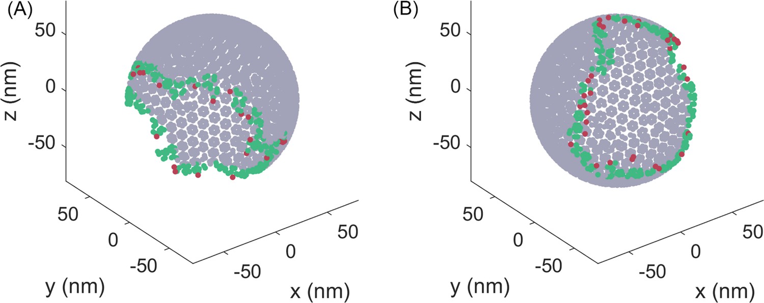
Characterizing bonds at the edge of the lattice.
Center-of-mass of each molecule is represented by a point. The green molecules are the molecules at the edge. A molecule is considered at the edge if it has less than 39 molecules within 15 nm. The red molecules are the molecules that have only a single bond to the lattice. The edge following our definition thus extends ~20 nm toward the interior of the lattice.
Figure 5 with 1 supplement
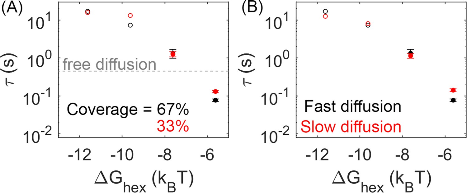
Lower lattice coverage or slower diffusion does not dramatically change the mean first-passage time (MFPT).
(A) First-passage time at different lattice coverages (67% and 33%). Closed circles are cases where Gag-Pol dimerization occurs in 100% of trajectories, while open circles are cases where Gag-Pol dimerization occurs in <100%. The gray line is the first-passage time when two free Gag-Pols diffusing on an empty spherical surface bind to one another. For the weakest lattice, rebinding is actually faster than diffusional encounter times between a dilute pair. (B) MFPT at different diffusion constants of the lipid. A monomer of Gag on the membrane diffuses at 0.2 µm2/s (black data), and diffuses slower as it grows in size consistent with Einstein-Stokes (Methods). We also simulated the system where diffusion of all species was slowed by a factor of 10 (red data). The MFPT is also not sensitive to changes in the dimer strength (Figure 5—figure supplement 1).
Figure 5—figure supplement 1

Effect of dimer interaction strength of mean first-passage time (MFPT) is minimal for these physiologic values.
Black data are from simulations with a dimer free energy of –11.62kBT, and red data are more stable at –13.62kBT. Unlike the effect of changing the hexamer free energy, as evidenced by the x-axis, a more stable dimer interaction has minimal effect on the MFPT. Filled data are from models where all trajectories produced dimerization events, open circles are lower bounds as not all trajectories produced events over the simulation time.
Figure 6
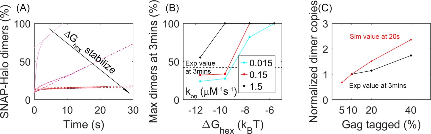
Analysis of our simulations mimics experimental biochemical measurements of Gag dimerization as a function of time, agreeing for moderately stable lattices.
(A) Percent of tagged Gag molecules that have formed a dimer (involving a SNAP-tag and HALO-tag plus linker) as a function of time. Here, 10% of Gag monomers were initially tagged either HALO or SNAP. As the hexamer stability ΔGhex increases, the dimerization yield dramatically slows. The dashed lines are linear fits of the last 1s of the curves. Results averaged over all 60 traces per parameter set. (B) Yield of dimers formed at 3 min estimated via simple linear extrapolation. Our results represent an upper bound. Dashed black line is the experimental measurement of the dimer formation at 3 min given 10% tagged populations. Fast (black), moderate (red), and slower (cyan) rate constants. With the most stable lattices and slowest rates, dimer yield is too low compared to experiment. (C) Dimer yield as we increase the population of initially tagged Gag monomers from 5% to 40%. Red is simulated yield at 20 s (to avoid extrapolation assumptions), and black is experimental yield at 3 min. We normalize the yield by the value at tagged Gag = 10%, given the different time points used.
Figure 7 with 2 supplements
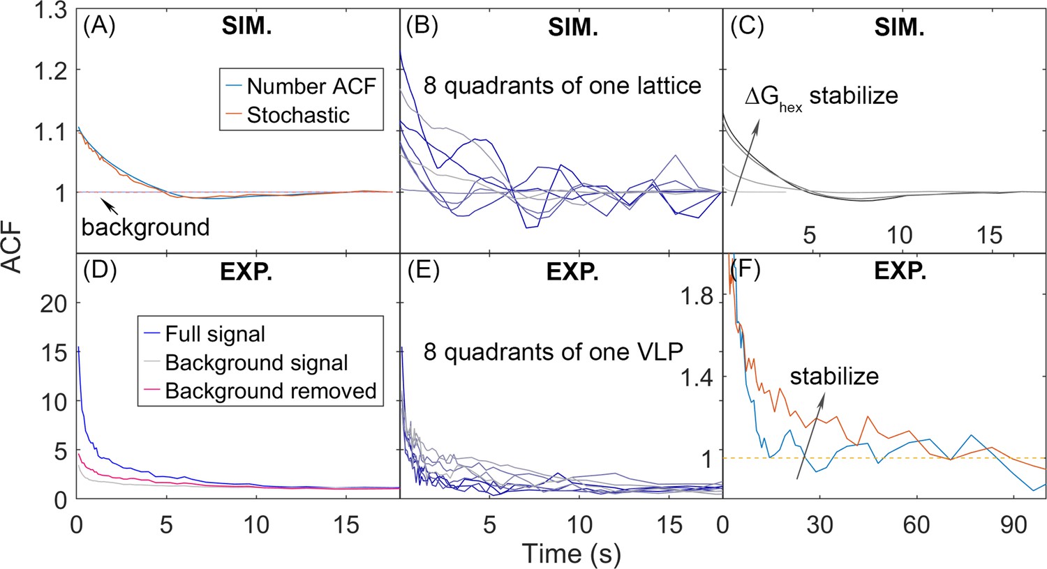
Autocorrelation functions (ACFs) of lattice dynamics from simulation and experiment show qualitatively similar trends.
(A) Number ACF of the simulations calculated directly from the copy numbers of Gag monomers shown in blue line. Averaged over all 8 quadrants over all 60 traces for one parameter set (see Methods). Using the stochastic localization method that mimics experiment shows excellent agreement (orange line). Dashed lines are the background signal, which is 1 as expected (bleaching of the Gag monomers causes limited drops in total copies across 20 s), as the total copy numbers across the membrane surface do not change. We note that the ACF values at our longest delays (i.e. τ>~10 s) are not statistically robust, because of the limited number of frames separated by these timescales. (B) ACF of each of the 8 quadrants of one simulated lattice. (C) As the lattice is stabilized by increasing ΔGhex, the ACF shows higher amplitude correlations that decay to 1 at longer times, additional trends shown in Figure 7—figure supplement 1. (D) ACF from stochastic localization experiments on Gag virus-like particles (VLPs). The blue curve is the average signal over all 8 quadrants over 11 VLPs. The gray is the background signal for the ACF of the total copy numbers across the surface, then averaged over all VLPs. The red line is the ACF signal after dividing out the background. (E) ACF of 8 quadrants of one experimental VLP. (F) The ACF from VLPs that have been stabilized with a fixative (orange curve) show the same trend as the stabilized lattices from simulation. The y-axis has been zoomed in to demonstrate the shift. The influence of experimental measurement noise on simulated ACFs is shown in Figure 7—figure supplement 2.
Figure 7—figure supplement 1

Autocorrelation functions (ACFs) at different free energies, reaction rates, diffusion, and surface coverage.
(A) The ACF amplitude increases at short times as the hexamer energy stabilizes, as (B) reaction rates slow, as (C) diffusion is faster, as (D) lattice coverage decreases. This is due to increased heterogeneity within the system leading to a larger variance in the copy numbers per quadrant.
Figure 7—figure supplement 2
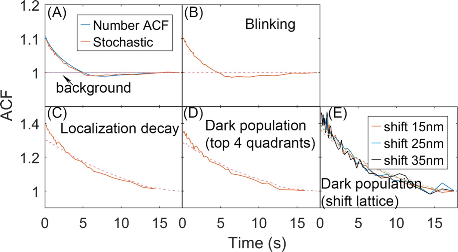
Effects of introduced noise on the autocorrelation functions (ACFs) calculated from stochastic localization measurements on simulation trajectories.
(A) From simulation we can directly count the number of monomers in each quadrant, and generate the complete number ACF. We can also perform a stochastic localization experiment, to mimic experiment, producing excellent agreement. In each frame, a monomer was localized here with 60% probability, pact = 0.6. Reducing the probability increases the noisiness of the ACF, but not its amplitude or timescales. No other ‘error’ was introduced into the localization measurement. For all plots, the background signal is shown in dashed red. The background is the correlation of the total copies counted across the full surface (no separation into quadrants). It is 1 as expected for the simulations due to conservation of total copies when no measurement noise is introduced. (B) For the stochastic localization, we add blinking of the fluorophore. Each molecule, once localized, can be localized again within the 10 frames (1s) since its first localization, with maximal three total localizations. Each molecule is on average localized twice, based on the experimental characterization of the Dendra fluorophore (Saha and Saffarian, 2020). (C) Here, we have the probability of localizing a molecule decays with time, pact = 0.6exp(−t/10), such that early on, more localizations occur than later on in the trajectory. This mimics a distribution of activation times for the fluorophores. (D) Here, we set the surface of the sphere is assumed to be only partially ‘visible’ to the laser. Here, only the top 4 quadrants are detected and analyzed, and the bottom 4 quadrants are ‘dark’. Those monomers in the bottom half become visible once they diffuse into the top hemisphere. (E) Similar to (D), except here the visible part of the sphere is asymmetric. The lattice is shifted to a distance along the x-axis and z-axis and only the molecules whose distance to the origin is less than Rsphere = 67 nm are visible. Monomers outside of that region are ‘dark’, until they diffuse into the visible part of the surface.
Videos
Video 1
Lattice dynamics for moderately stable dynamics that are consistent with structural and biochemical experiments.
. ka2D (nm2/μs)=2.5 × 10–2; gap between each frame: 10 ms; overall time length: 20 s.
Video 2
Lattice dynamics for an unstable lattice.
. ka2D (nm2/μs)=2.5 × 10–2; gap between each frame: 10 ms; overall time length: 4.5 s.
Video 3
Lattice dynamics for a more highly stable lattice with slower binding kinetics.
. ka2D (nm2/μs)=2.5 × 10–3; gap between each frame: 10 ms; overall time length: 20 s.
Tables
Table 1
Simulation parameters for remodeling dynamics.
| Gag copy number | ~2500 | ||
| Gag-Pol copy number | ~125 | ||
| Lipid copy number | 4000 | ||
| Radius of sphere | 67 nm | ||
| Time-step | 0.2 μs | ||
| ka2D (nm2/μs), ka3D (M–1s–1), kb Gag-Mem | 1, 1.2×10⁶, 0.61 s–1 | ||
| ka2D (nm2/μs) Gag-Gag dimer | 2.5×10⁻³ | 2.5×10⁻² | 2.58×10⁻¹ |
| ka2D (nm2/μs) Gag-Gag hexamer | 2.5×10⁻³ | 2.5×10⁻² | 2.737×10⁻¹ |
| ka3D (M–1s–1) Gag-Gag hexamer | 1.5×10⁴ | 1.5×10⁵ | 1.6×10⁶ |
| kb Gag-Gag dimer (s–1) (–11.62kBT) | 1.35×10⁻¹ s–1 | 1.35×100 | 1.4×101 |
| kb Gag-Gag dimer (s–1) (–13.62kBT) | 1.8×10⁻² s–1 | 1.8×10⁻¹ | 1.89×100 |
| kb Gag-Gag hexamer (s–1) (–5.62kBT) | 5.45×101 | 5.5×10² | 6.01×10³ |
| kb Gag-Gag hexamer (s–1) (–7.62kBT) | 7.37×100 | 7.44×101 | 8.13×10² |
| kb Gag-Gag hexamer (s–1) (–9.62kBT) | 1.0×100 | 1.0×101 | 1.1×10² |
| kb Gag-Gag hexamer (s–1) (–11.62kBT) | 1.35×10⁻¹ | 1.36×100 | 1.49×101 |
| ΔGstrain | 2.3kBT | ||
Additional files
Download links
A two-part list of links to download the article, or parts of the article, in various formats.
Downloads (link to download the article as PDF)
Open citations (links to open the citations from this article in various online reference manager services)
Cite this article (links to download the citations from this article in formats compatible with various reference manager tools)
Structure of the HIV immature lattice allows for essential lattice remodeling within budded virions
eLife 12:e84881.
https://doi.org/10.7554/eLife.84881


