Eelbrain, a Python toolkit for time-continuous analysis with temporal response functions
Figures
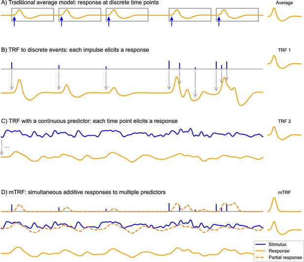
The convolution model for brain responses as a generalization of the averaging-based paradigm.
(A) The traditional event-related analysis method assumes that each stimulus (blue arrows) evokes an identical, discrete response, and this response can be recovered by averaging. This model assumes that responses are clearly separated in time. (B) In contrast, the convolution model assumes that each time point in the stimulus could potentially evoke a response. This is implemented with time series predictor variables, illustrated here with a time series containing several impulses. These impulses represent discrete events in the stimulus that are associated with a response, for example, the occurrence of words. This predictor time series is convolved with some kernel characterizing the general shape of responses to this event type – the temporal response function (TRF), depicted on the right. Gray arrows illustrate the convolution, with each impulse producing a TRF-shaped contribution to the response. As can be seen, the size of the impulse determines the magnitude of the contribution to the response. This allows testing hypotheses about stimulus events that systematically differ in the magnitude of the responses they elicit, for example, that responses increase in magnitude the more surprising a word is. A major advantage over the traditional averaging model is that responses can overlap in time. (C) Rather than discrete impulses, the predictor variable in this example is a continuously varying time series. Such continuously varying predictor variables can represent dynamic properties of sensory input, for example: the acoustic envelope of the speech signal. The response is dependent on the stimulus in the same manner as in (B), but now every time point of the stimulus evokes its own response shaped like the TRF and scaled by the magnitude of the predictor. Responses are, therefore, heavily overlapping. (D) The multivariate TRF (mTRF) model is a generalization of the TRF model with multiple predictors: like in a multiple regression model, each time series predictor variable is convolved with its own corresponding TRF, resulting in multiple partial responses. These partial responses are summed to generate the actual complete response. Source code: figures/Convolution.py.
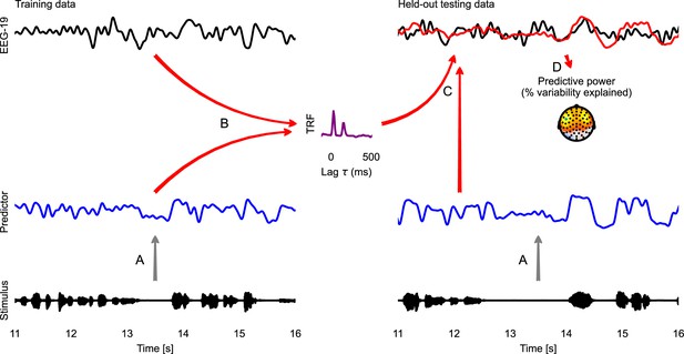
Temporal response function (TRF) analysis of EEG speech tracking.
The left half illustrates the estimation of a TRF model, the right half the evaluation of this model with cross-validation. First, the stimulus is used to generate a predictor variable, here the acoustic envelope (A). The predictor and corresponding EEG data (here only one sensor is shown) are then used to estimate a TRF (B). This TRF is then convolved with the predictor for the held-out testing data to predict the neural response in the testing data (C; measured: black; predicted: red). This predicted response is compared with the actual, measured EEG response to evaluate the predictive power of the model (D). A topographic map shows the % of the variability in the EEG response that is explained by the TRF model, estimated independently at each sensor. This head-map illustrates how the predictive power of a predictor differs across the scalp, depending on which neural sources a specific site is sensitive to. The sensor whose data and TRF are shown is marked in green. Source code: figures/TRF.py.
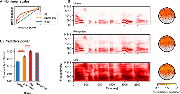
Nonlinear response scales.
(A) Illustration of logarithmic and power-law scales, compared to linear scale. (B) Gammatone spectrograms were ransformed to correspond to linear, power-law, and logarithmic response scales. Topographic maps show the predictive power of the three different spectrogram models. The color represents the percent of the variability in the EEG data that is explained by the respective multivariate TRF (mTRF) model. (C) Statistical comparison of the predictive power, averaged across all sensors. Error bars indicate the within-subject standard error of the mean, and significance is indicated for pairwise t-tests (df = 32). ***p≤0.001; Source code: figures/Auditory-scale.py.
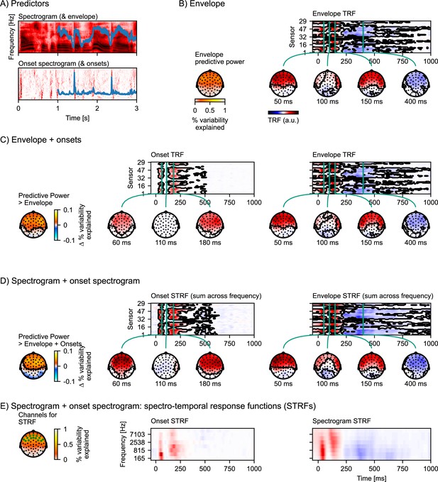
Auditory temporal response functions.
(A) Common representations of auditory speech features: an auditory spectrogram (upper panel), and the acoustic envelope, tracking total acoustic energy across frequencies over time (blue line); and an acoustic onset spectrogram (lower panel), also with a one-dimensional summary characterizing the presence of acoustic onsets over time (blue line). (B) Brain responses are predicted from the acoustic envelope of speech alone. Left: Cross-validated predictive power is highly significant (p<0.001) at a large cluster covering all sensors. Right: the envelope temporal response function (TRF) – the y-axis represents the different EEG channels (in an arbitrary order), and the x-axis represents predictor-response time lags. The green vertical lines indicate specific (manually selected) time points of interest, for which head map topographies are shown. The black outlines mark significant clusters (p≤0.05, corrected for the whole TRF). For the boosting algorithm, predictors and responses are typically normalized, and the TRF is analyzed and displayed in this normalized scale. (C) Results for an multivariate TRF (mTRF) model including the acoustic envelope and acoustic onsets (blue lines in A). The left-most head map shows the percentage increase in predictive power over the TRF model using just the envelope (p<0.001; color represents the change in the percent variability explained; black outlines mark significant clusters, p≤0.05, family-wise error corrected for the whole head map). Details are analogous to (B). (D) Results for an mTRF model including spectrogram and onset spectrogram, further increasing predictive power over the one-dimensional envelope and onset model (p<0.001; color represents the change in percent variability explained). Since the resulting mTRFs distinguish between different frequencies in the stimulus, they are called spectro-temporal response functions (STRFs). In (D), these STRFs are visualized by summing across the different frequency bands. (E) To visualize the sensitivity of the STRFs to the different frequency bands, STRFs are instead averaged across sensors sensitive to the acoustic features. The relevant sensors are marked in the head map on the left, which also shows the predictive power of the full spectro-temporal model (color represents the percent variability explained). Because boosting generates sparse STRFs, especially when predictors are correlated, as are adjacent frequency bands in a spectrogram, STRFs were smoothed across frequency bands for visualization. a.u.: arbitrary units. Source code: figures/Auditory-TRFs.py.
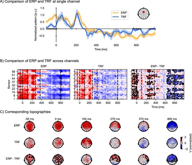
Temporal response functions (TRFs) to discrete events are similar to event-related potentials (ERPs), but control for acoustic processing and overlapping responses.
To visualize ERP and TRF on a similar scale, both ERP and TRF were normalized (parametric normalization). (A) Visualization of the ERP and TRF response over time for a frontocentral channel, as indicated on the inset. The gray bars on the time axis indicate the temporal clusters in which the ERP and TRF differ significantly. Shading indicates within-subject standard errors (n = 33). (B) Visualization of ERP and TRF responses across all channels: the ERP responses to word onsets (left), the TRF to word onsets while controlling for acoustic processing (middle), and the difference between the ERP and the TRF (right). The black outline marks clusters in which the ERP and the TRF differ significantly in time and across sensors, assessed by a mass-univariate related-measures t-test. (C) Visualization of the topographies at selected time points, indicated by the vertical, dashed lines in (B), for respectively the ERP (top row), TRF (middle row), and their difference (bottom row). The contours mark regions where the ERP differs significantly from the TRF, as determined by the same mass-univariate related-measures t-test as in (B). a.u.: arbitrary units. Source code: figures/Comparison-ERP-TRF.py.
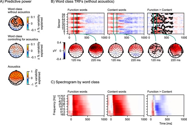
The difference in response to content and function words explained by acoustic differences.
(A) Model comparisons of predictive power across the scalp. Each plot shows a head-map of the change in predictive power between different pairs of models. Top: Equation 5 > Equation 6; middle: Equation 7 > Equation 4; bottom: Equation 4 > Equation 6. Color represents the difference in percent variability explained. (B) Brain responses occurring after function words differ from brain responses after content words. Responses were estimated from the temporal response functions (TRFs) of model Equation 5 by adding the word-class-specific TRF to the all words TRF. The contours mark the regions that are significantly different between function and content words based on a mass-univariate related-measures t-test. (C) Function words are associated with a sharper acoustic onset than content words. The average spectrograms associated with function and content words were estimated with time-lagged regression, using the same algorithm also used for TRF estimation, but predicting the acoustic spectrogram from the function and content word predictors. A dotted line is plotted at 70 ms to help visual comparison. Color scale is normalized. Source code: figures/Word-class-acoustic.py.
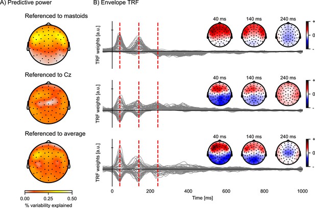
Comparison of EEG reference strategies.
Predictive power topographies and temporal response functions (TRFs) to the acoustic envelope, according to three different referencing strategies: the average of the left and right mastoids (top), the central electrode Cz (middle), and the common average (bottom). (A) Visualization of the predictive power obtained with the different referencing strategies (color represents the percent variability explained). (B) The envelope TRFs for the different referencing strategies. The insets indicate the topographies corresponding to the vertical red dashed lines at latencies of 40, 140, and 240 ms. Source code: figures/Reference-strategy.py.
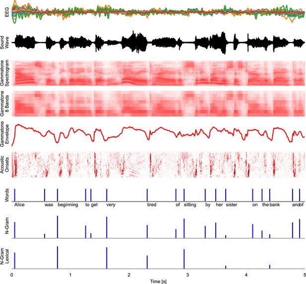
Time series representations of different commonly used speech representations, aligned with the EEG data.
EEG: band-pass filtered EEG responses. Sound Wave: acoustic wave form, time-aligned to the EEG data. Gammatone Spectrogram: spectrogram representation modeling processing at the auditory periphery. Gammatone 8 Bands: the gammatone spectrogram binned into 8 equal-width frequency bins for computational efficiency. Gammatone Envelope: sum of the gammatone spectrogram across all frequency bands, reflecting the broadband acoustic envelope. Acoustic Onsets: acoustic onset spectrogram, a transformation of the gammatone spectrogram using a neurally inspired model of auditory edge detection. Words: a uniform impulse at each word onsets, predicting a constant response to all words. N-Gram: an impulse at each word onset, scaled with that word’s surprisal, estimated from an n-gram language model. This predictor will predict brain responses to words that scale with how surprising each word is in its context. N-Gram Lexical: N-Gram surprisal only at content words, predicting a response that scales with surprisal and occurs at content words only. Source code: figures/Time-series.py.
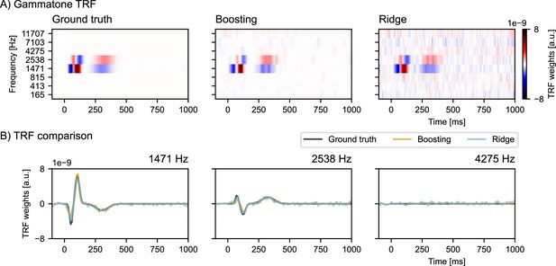
Simulation study comparing boosting with ridge regression when modeling multiple correlated variables.
(A) A pre-defined multivariate temporal response functions (mTRF) was used to generate simulated EEG data (left panel), and then reconstructed by boosting and ridge regression (middle and right panel). (B) Overlays of boosting, ridge regression, and ground truth TRFs at different center frequencies for comparison. Note that the ridge TRF follows the ground truth closely, but produces many false positives. On the contrary, the boosting TRF enjoys an excellent true negative rate, at the expense of biasing TRF peaks and troughs toward 0. a.u.: arbitrary units. Source code: figures/Collinearity.py.
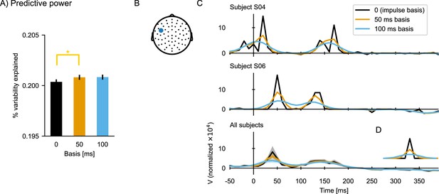
The effect of using a basis function for temporal response function (TRF) estimation.
(A) Predictive power of the TRFs estimated with different basis windows (expressed as a percent of the variability in the EEG data that is explained by the respective TRF model). Error bars indicate the within-subject standard error of the mean, and significance is indicated for pairwise t-tests (df = 32; *p≤0.05). (B) The sensor selected for illustrating the TRFs. (C) TRFs for two subject (upper and middle plots) and the average across all subjects (bottom). (D) Basis windows. Notice that the impulse basis (‘0’) is only a single sample wide, but it appears as a triangle in a line plot with the apparent width determined by the sampling rate. Source code: figures/TRF-Basis.py.


