Cell type-specific connectome predicts distributed working memory activity in the mouse brain
- Center for Neural Science, New York University, United States
- Bristol Computational Neuroscience Unit, School of Engineering Mathematics and Technology, University of Bristol, United Kingdom
- Campus Institute for Dynamics of Biological Networks, University of Göttingen, Germany
- The Key Laboratory of Biomedical Information Engineering of Ministry of Education,Institute of Health and Rehabilitation Science,School of Life Science and Technology, Research Center for Brain-inspired Intelligence, Xi’an Jiaotong University, China
Figures
Figure 1 with 1 supplement
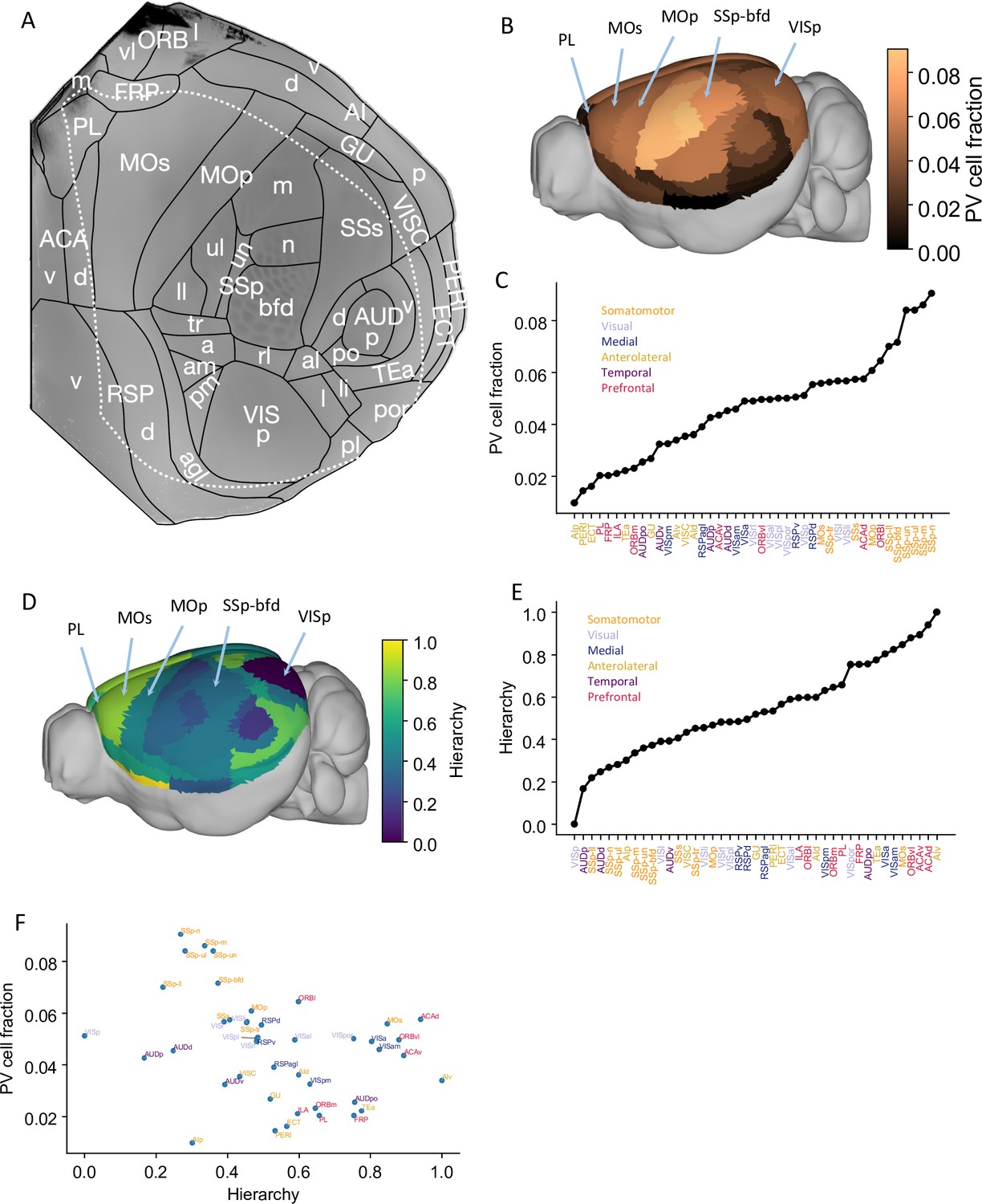
Anatomical basis of the multiregional mouse cortical model.
(A) Flattened view of mouse cortical areas. Figure adapted from Harris et al., 2019. (B) Normalized parvalbumin (PV) cell fraction for each brain area, visualized on a 3D surface of the mouse brain. Five areas are highlighted: VISp, primary somatosensory area, barrel field (SSp-bfd), primary motor (MOp), MOs, and PL. (C) The PV cell fraction for each cortical area, ordered. Each area belongs to one of five modules, shown in color (Harris et al., 2019). (D) Hierarchical position for each area on a 3D brain surface. Five areas are highlighted as in (B), and color represents the hierarchy position. (E) Hierarchical positions for each cortical area. The hierarchical position is normalized and the hierarchical position of VISp is set to be 0. As in (C), the colors represent the module that an area belongs to. (F) Correlation between PV cell fraction and hierarchy (Pearson correlation coefficient r = –0.35, p<0.05).
© 2019, Harris et al. Panel A is reproduced from Figure 1b of Harris et al., 2019 with permission. It is not covered by the CC-BY 4.0 licence and further reproduction of this panel would need permission from the copyright holder.
Figure 1—figure supplement 1

Anatomical details of the mouse cortex.
(A) Connectivity matrix depicting cortico-cortical connections between 43 cortical areas. Areas are sorted according to their hierarchy. (B) The raw parvalbumin (PV) cell density for each cortical area (Y-axis), with areas sorted (X-axis). Each area belongs to one of five modules, shown in color (see also Figure 1; Harris et al., 2019). (C) Neuron density for each cortical area with same sorted order as (B). The data is from Erö et al., 2018.
Figure 2 with 1 supplement
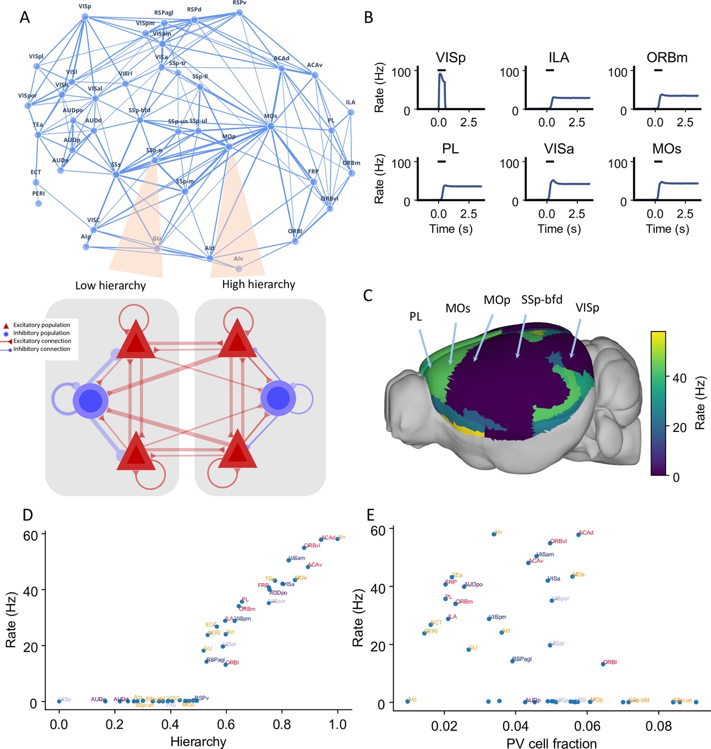
Distributed working memory activity depends on the gradient of parvalbumin (PV) interneurons and the cortical hierarchy.
(A) Model design of the large-scale model for distributed working memory. Top: connectivity map of the cortical network. Each node corresponds to a cortical area and an edge is a connection, where the thickness of the edge represents the strength of the connection. Only strong connections are shown (without directionality for the sake of clarity). Bottom: local and long-range circuit design. Each local circuit contains two excitatory populations (red), each selective to a particular stimulus and one inhibitory population (blue). Long-range connections are scaled by mesoscopic connectivity strength (Oh et al., 2014) and follows counterstream inhibitory bias (CIB) (Mejías and Wang, 2022). (B) The activity of six selected areas during a working memory task is shown. A visual input of 500 ms is applied to area VISp, which propagates to the rest of the large-scale network. (C) Delay-period firing rate for each area on a 3D brain surface. Similar to Figure 1B, the positions of five areas are labeled. (D) Delay-period firing rate is positively correlated with cortical hierarchy (r = 0.91, p<0.05). (E) Delay-period firing rate is negatively correlated with PV cell fraction (r = –0.43, p<0.05).
Figure 2—figure supplement 1
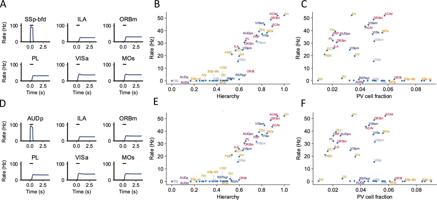
Example simulation for different sensory modalities.
The simulation protocol is the same as the default one in Figure 2, except that the external input is applied to primary sensory areas related to two other sensory modalities: somatosensory and auditory. (A) The activity of six selected areas during the working memory task is shown. A somatosensory input of 500 ms is applied to primary somatosensory area SSp-bfd, which propagates to the rest of the large-scale network. (B) Similar to the simulation where a primary visual area is stimulated (Figure 2D), delay-period firing for somatosensory stimulation is positively correlated with cortical hierarchy (r = 0.89, p<0.05). (C) Delay-period firing rate is moderately correlated with parvalbumin (PV) cell fraction (r = –0.4, p<0.05). (D), (E), and (F) are similar to (A), (B), and (C) except that the input is given to primary auditory area AUDp. (E) Delay-period firing is also positively correlated with cortical hierarchy (r = 0.89, p<0.05). (F) Delay-period firing rate is moderately correlated with PV cell fraction (r = –0.4, p<0.05).
Figure 3 with 1 supplement
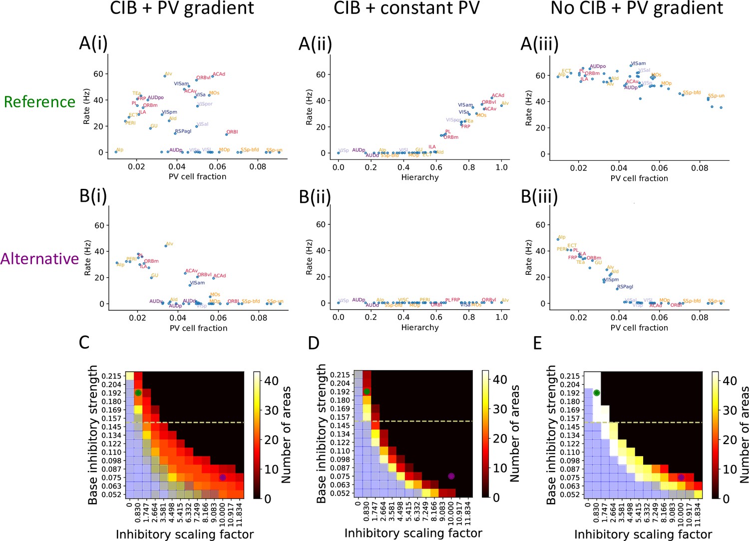
The role of parvalbumin (PV) inhibitory gradient and hierarchy-based counter inhibitory bias (CIB) in determining persistent activity patterns in the cortical network.
(A(i)) Delay firing rate as a function of PV cell fraction with both CIB and PV gradient present (r = –0.42, p<0.05). This figure panel is the same as Figure 2E. (A(ii)) Delay firing rate as a function of hierarchy after removal of PV gradient (r = –0.85, p<0.05). (A(iii)) Delay firing rate as a function of PV cell fraction after removal of CIB (r = –0.74, p<0.05). (B(i)) Delay firing rate as a function of PV cell fraction with both CIB and PV gradient present, in the alternative regime (r = –0.7, p<0.05). (B(ii)) Delay firing rate as a function of hierarchy after removal of PV gradient, in the alternative regime (r = –0.95, p<0.05). (B(iii)) Delay firing rate as a function of PV cell fraction after removal of CIB, in the alternative regime (r = –0.84, p<0.05). (C–E) Number of areas showing persistent activity (color coded) as a function of the local inhibitory gradient (, X-axis) and the base value of the local inhibitory gradient (, Y-axis) for the following scenarios: (C) CIB and PV gradient, (D) with PV gradient replaced by a constant value, and (E) with CIB replaced by a constant value. The reference regime is located at the top-left corner of the heatmap (green dot) and corresponds to A(i)–A(iii), while the alternative regime is located at the lower-right corner (purple dot) and corresponds to B(i)–B(iii). The yellow dashed lines separate parameters sets for which none of the areas show ‘independent’ persistent activity (above the line) from parameter sets for which some areas are capable of maintaining persistent activity without input from other areas (below the line). Blue shaded squares in the heatmap mark the absence of a stable baseline.
Figure 3—figure supplement 1
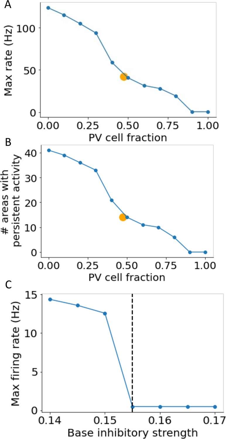
Dependence of persistent activity on inhibitory model parameters.
(A) The maximum firing rate of all areas depends on the constant parvalbumin (PV) cell fraction in models without a gradient of PV. Average PV cell fraction from the anatomical data is shown as an orange dot. (B) Same as (A), except for the number of areas showing persistent activity. (C) Firing rate during the delay period for local circuits without long-range projections as a function of base inhibitory strength. If the base inhibitory strength is larger than a threshold (0.155, marked by the dashed line), none of the areas show independent persistent activity.
Figure 4
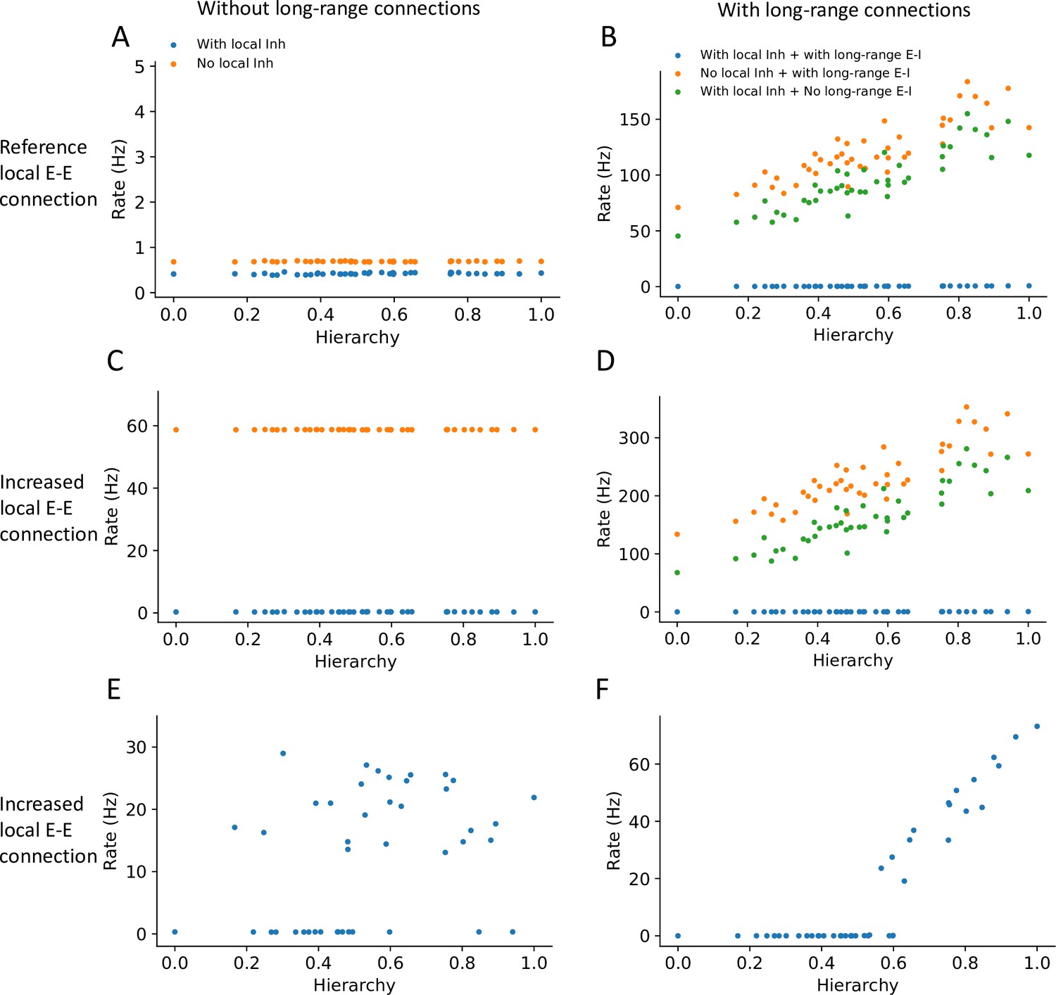
Local and long-range projections modulate the baseline stability of individual cortical areas.
Steady state firing rates are shown as a function of hierarchy for different scenarios: (A) without long-range connections in the reference regime (, ), (B) with long-range connections in the reference regime (), (C) without long-range connections and increased local excitatory connections (, ), and (D) with long-range connections (increased long-range connections to excitatory neurons, ) and increased local excitatory connections. (E) Firing rate as a function of hierarchy when external input given to each area, showing bistability for a subset of areas (parameters as in (C) and ’with local inh’). (F) Firing rate as a function of hierarchy when external input is applied to area VISp (parameters as in (D) and ’with local inh + with long-range E-I’).
Figure 5 with 1 supplement
Thalamocortical interactions help maintain distributed persistent activity.
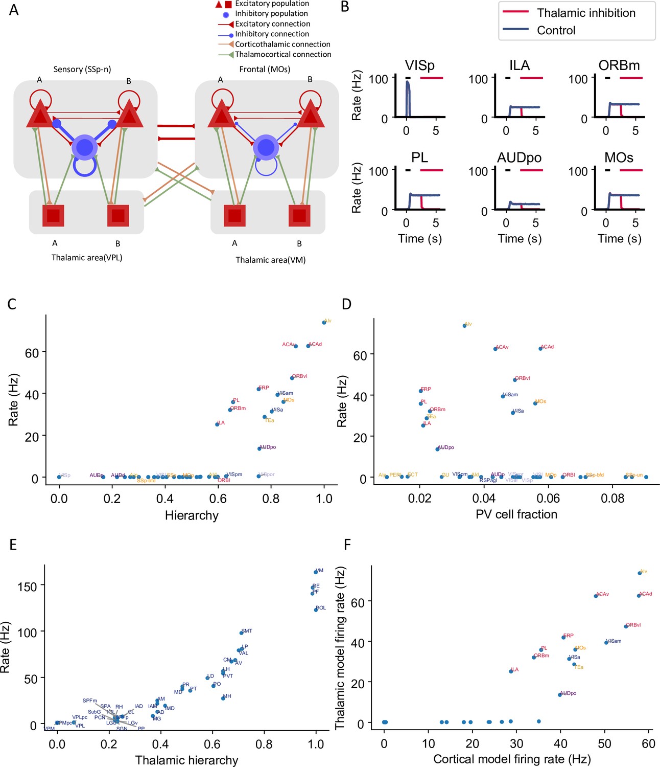
(A) Model schematic of the thalamocortical network. The structure of the cortical component is the same as our default model in Figure 2A, but with modified parameters. Each thalamic area includes two excitatory populations (red square) selective to different stimuli. Long-range projections between thalamus and cortex also follow the counterstream inhibitory bias rule as in the cortex. Feedforward projections target excitatory neurons with stronger connections and inhibitory neurons with weaker connections; the opposite holds for feedback projections. (B) The activity of six sample cortical areas in a working memory task is shown during control (blue) and when thalamic areas are inhibited in the delay period (red). Black dashes represent the external stimulus applied to VISp. Red dashes represent external inhibitory input given to all thalamic areas. (C) Delay-period firing rate of cortical areas in the thalamocortical network. The activity pattern has a positive correlation with cortical hierarchy (r = 0.78, p<0.05). (D) Same as (C) but plotted against parvalbumin (PV) cell fraction. The activity pattern has a negative correlation with PV cell fraction, but it is not significant (r = –0.26, p=0.09). (E) Delay firing rate of thalamic areas in thalamocortical network. The firing rate has a positive correlation with thalamic hierarchy (r = 0.94, p<0.05). (F) Delay-period firing rate of cortical areas in thalamocortical network has a positive correlation with delay firing rate of the same areas in a cortex-only model (r = 0.77, p<0.05). Note that only the areas showing persistent activity in both models are considered for correlation analyses.
Figure 5—figure supplement 1
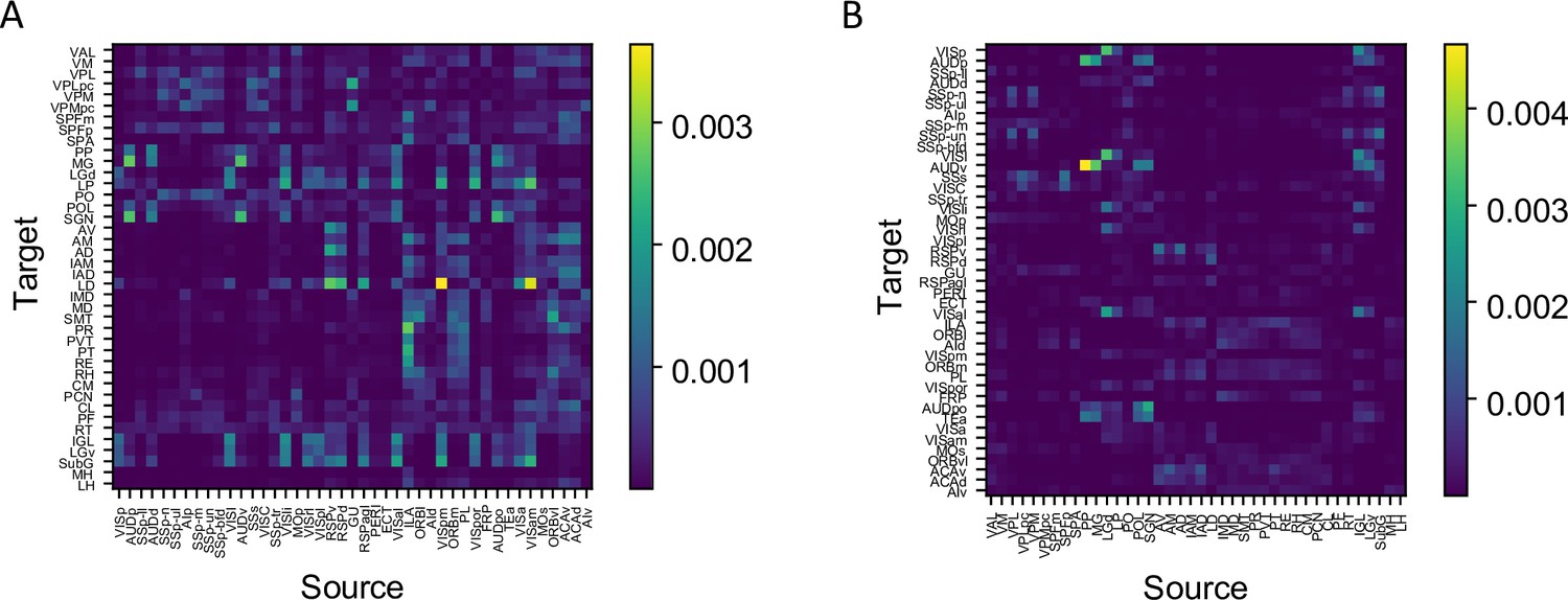
Anatomical data of thalamus and cortical connectivity.
(A) Connectivity matrix of corticothalamic connections: 43 cortical areas to 40 thalamic areas. (B) Connectivity matrix of thalamocortical connections: 40 thalamic areas to 43 cortical areas.
Figure 6 with 3 supplements
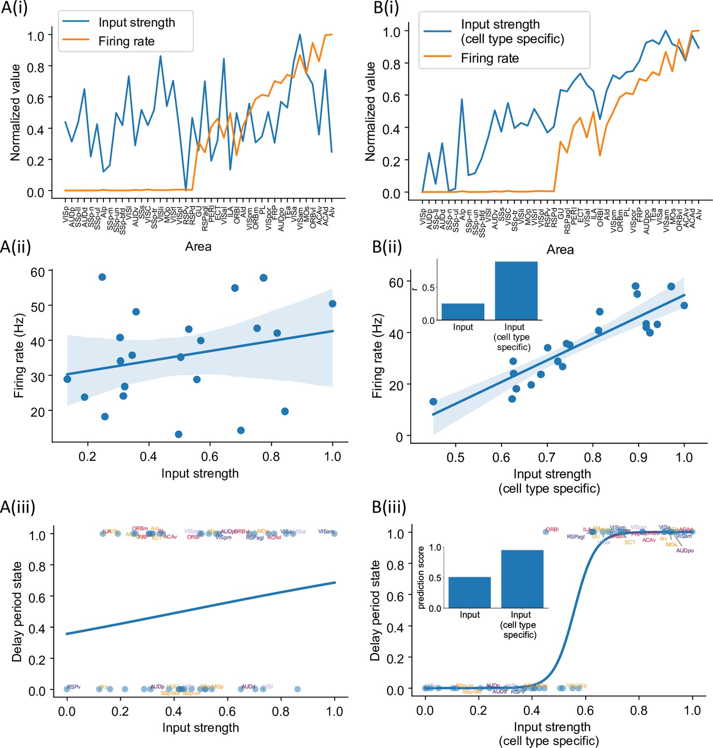
Cell type-specific connectivity measures are better at predicting firing rate pattern than nonspecific ones.
(A(i)) Delay-period firing rate (orange) and input strength for each cortical area. Input strength of each area is the sum of connectivity weights of incoming projections. Areas are plotted as a function of their hierarchical positions. Delay-period firing rate and input strength are normalized for better comparison. (A(ii)) Input strength does not show significant correlation with delay-period firing rate for areas showing persistent activity in the model (r = 0.25, p=0.25). (A(iii)) Input strength cannot be used to predict whether an area shows persistent activity or not (prediction accuracy = 0.51). (B(i)) Delay-period firing rate (orange) and cell type-specific input strength for each cortical area. Cell type-specific input strength considers how the long-rang connections target different cell types and is the sum of modulated connectivity weights of incoming projections. Same as (A(i)), areas are sorted according to their hierarchy and delay-period firing rate and input strength are normalized for better comparison. (B(ii)) Cell type-specific input strength has a strong correlation with delay-period firing rate of cortical areas showing persistent activity (r = 0.89, p<0.05). Inset: comparison of the correlation coefficient for raw input strength and cell type-specific input strength. (B(iii)) Cell type-specific input strength predicts whether an area shows persistent activity or not (prediction accuracy = 0.95). Inset: comparison of the prediction accuracy for raw input strength and cell type-specific input strength.
Figure 6—figure supplement 1
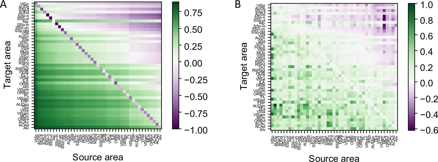
Details of cell type-specific connectivity measures.
(A) The matrix of cell type projection coefficients between cortical areas. The cell type projection coefficient is given by the formula . (B) The matrix of connectivity strengths, modified by cell type projection coefficient between cortical areas. The modified connectivity strength is given by .
Figure 6—figure supplement 2
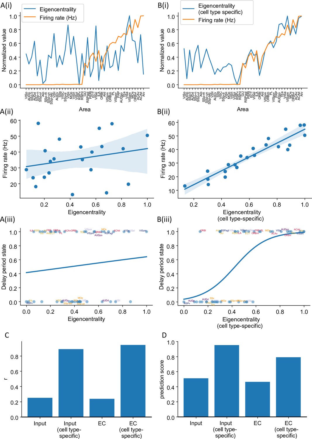
Cell type-specific eigenvector centrality measures are better at predicting firing rate patterns than raw eigenvector centrality measures.
The analysis is the same as in Figure 6, where we compared cell type-specific input strength and raw input strength. Eigenvector centrality (EC, eigencentrality) of area is the ith element of the leading eigenvector of the connectivity matrix. It quantifies how many areas are connected with the target area and how important are these neighbors. Details are given in the ‘Methods’ section. (A(i)) Delay-period firing rate (orange) and eigenvector centrality for each cortical area (blue). (A(ii)) Eigenvector centrality does not show a significant correlation with delay-period firing rate for areas showing persistent activity in the model (r = 0.24, p=0.29). (A(iii)) Eigenvector centrality cannot be used to predict whether an area shows persistent activity or not (prediction accuracy = 0.46). (B(i)) Delay-period firing rate (orange) and cell type-specific eigenvector centrality for each cortical area (blue). (B(ii)) Cell type-specific eigenvector centrality has a strong correlation, with the firing rate of cortical areas showing persistent activity (r = 0.94, p<0.05). (B(iii)) Cell type-specific eigenvector centrality predicts whether an area shows persistent activity or not (prediction accuracy = 0.79). (C) Comparison of the correlation coefficient r for raw eigenvector centrality and cell type-specific eigenvector centrality in predicting delay firing rate. Raw input strength and cell type-specific input strength are also included for comparison. (D) Comparison of the prediction accuracy for raw eigenvector centrality and cell type-specific eigenvector centrality. Raw input strength and cell type-specific input strength are also included for comparison.
Figure 6—figure supplement 3
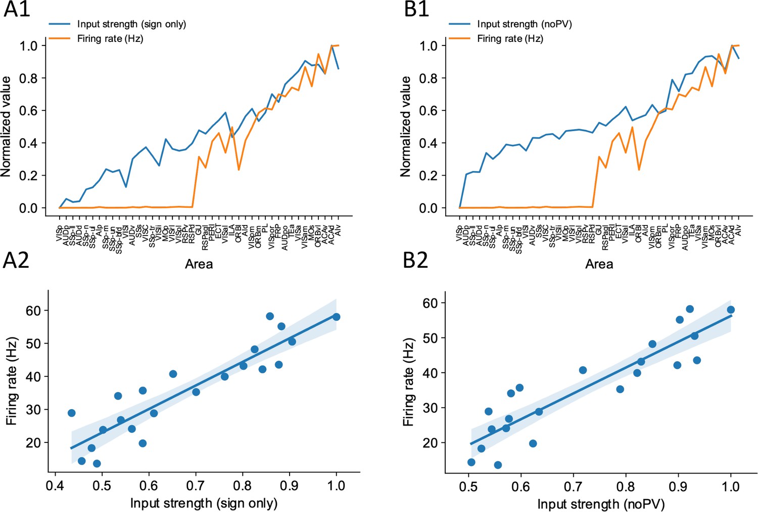
Sign-only input strength measure and noPV input strength measure predict firing rate well.
(A1) Delay-period firing rate (orange) and sign-only input strength for each cortical areas. (A2) Sign-only input strength has a strong correlation with delay-period firing rate of cortical areas showing persistent activity (r = 0.90, p<0.05). (B1) Delay-period firing rate (orange) and noPV input strength for each cortical areas. (B2) noPV input strength has a strong correlation with delay-period firing rate of cortical areas showing persistent activity (r = 0.90, p<0.05).
Figure 7 with 1 supplement
A core subnetwork generates persistent activity across the cortex.
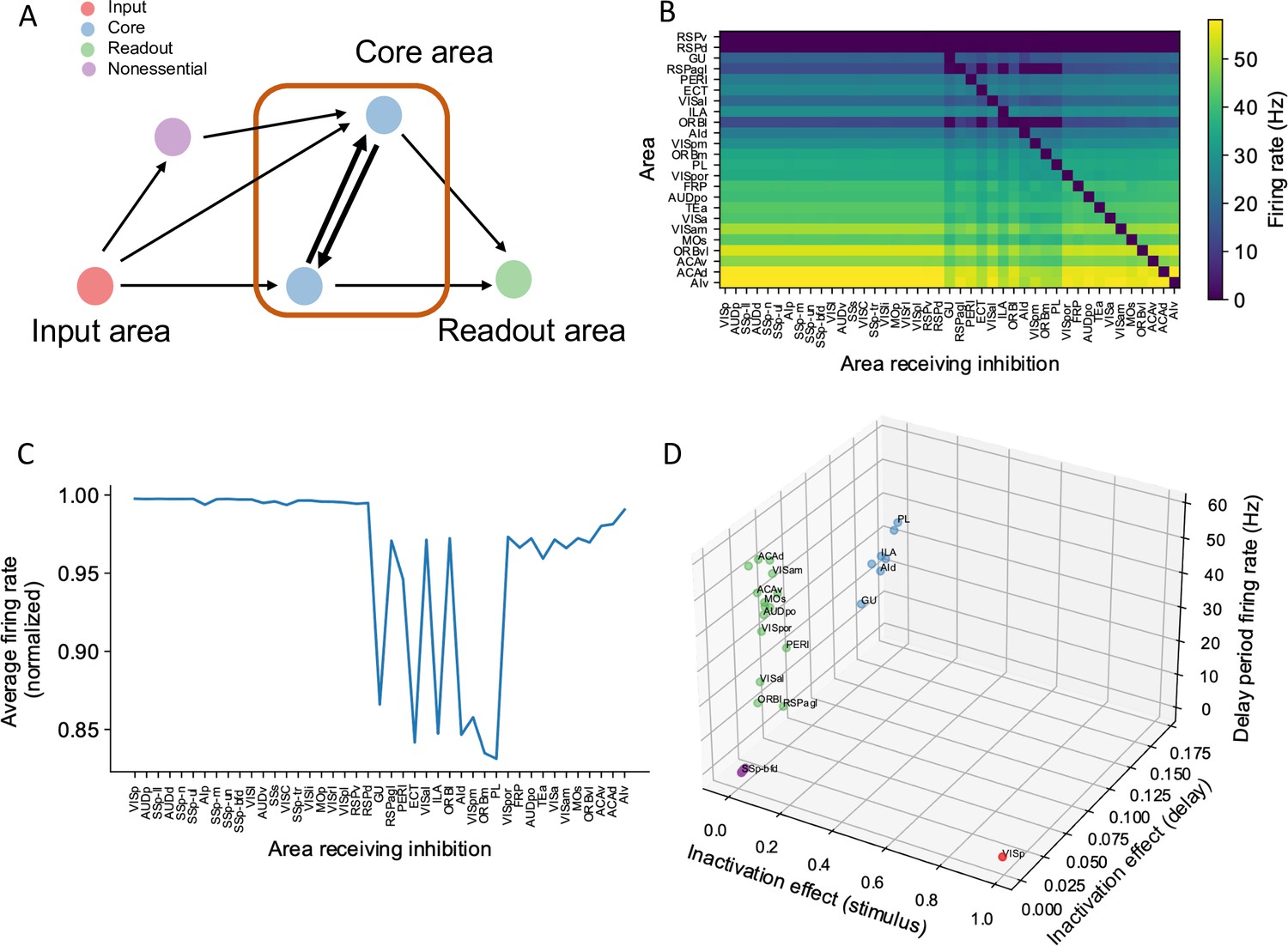
(A) We propose four different types of areas. Input areas (red) are responsible for coding and propagating external signals, which are then propagated through synaptic connections. Core areas (blue) form strong recurrent loops and generate persistent activity. Readout areas (green) inherit persistent activity from core areas. Nonessential areas (purple) may receive inputs and send outputs but they do not affect the generation of persistent activity. (B) Delay-period firing rate for cortical areas engaged in working memory (Y-axis) after inhibiting different cortical areas during the delay period (X-axis). Areas in the X-axis and Y-axis are both sorted according to hierarchy. Firing rates of areas with small firing rate (<1 Hz) are partially shown (only RSPv and RSPd are shown because their hierarchical positions are close to areas showing persistent activity). (C) The average firing rate for areas engaged in persistent activity under each inhibition simulation. The X-axis shows which area is inhibited during the delay period, and the Y-axis shows the average delay period activity for all areas showing persistent activity. Note that when calculating the average firing rate, the inactivated area was excluded in order to focus on the inhibition effect of one area on other areas. Average firing rates on the Y-axis are normalized using the average firing in control (no inhibition) simulation. (D) Classification of four types of areas based on their delay period activity after stimulus- and delay-period inhibition (color denotes the type for area, as in A). The inhibition effect, due to either stimulus or delay period inhibition, is the change of average firing rate normalized by the average firing rate in the control condition. Areas with strong inhibition effect during stimulus period are classified as input areas; areas with strong inhibition effect during delay period and strong delay-period firing rate are classified as core areas; areas with weak inhibition effect during delay period but strong delay-period firing rate during control are classified as readout areas; and areas with weak inhibition effect during delay period and weak delay-period firing rate during control are classified as nonessential areas.
Figure 7—figure supplement 1
Multiple-area inhibition experiments demonstrate the relative importance for core and readout areas in maintaining network-level persistent activity.
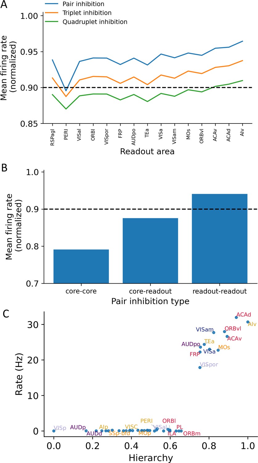
(A) The X-axis shows readout areas that are inhibited as part of a pair (blue), triplet (orange), or quadruplet (green). For any given readout area A, the Y-axis shows the average firing rate of all cortical areas that exhibit persistent activity when A was inhibited as part of the inhibited pair (triplet, quadruplet). The decrement in delay period activity is stronger as more areas are inhibited. (B) Bar plots showing the average firing rate of the network after inhibition of pairwise combinations of core and readout areas. For example, the bar plot for ’readout-readout’ is the average firing rate for all readout-readout areas pairs and is corresponding to the blue curve in (A). Dashed lines in (A) and (B) denote a threshold below which we consider an ’inhibition effect’ to be significant. (C) Delay-period firing rates as a function of hierarchy after inhibition of all core areas during the delay period. Although some readout areas show persistent firing, there is 48% decrement in average firing rate.
Figure 8 with 2 supplements
The core subnetwork can be identified structurally by the presence of strong excitatory loops.
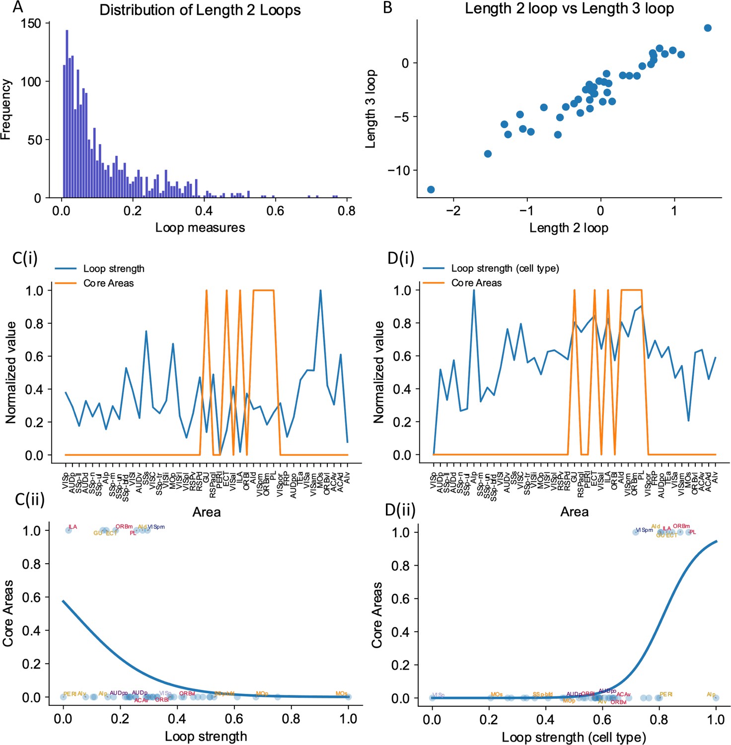
(A) Distribution of length 2 loops. X-axis is the single-loop strength of each loop (product of connectivity strengths within loop) and Y-axis is their relative frequency. (B) Loop strengths of each area calculated using different length of loops (e.g., length 3 vs length 2) are highly correlated (r = 0.96, p<0.05). (C(i)) Loop strength (blue) is plotted alongside core areas (orange), a binary variable that takes the value 1 if the area is a core area, 0 otherwise. Areas are sorted according to their hierarchy. The loop strength is normalized to a range of (0, 1) for better comparison. (C(ii)) A high loop strength value does not imply that an area is a core area. Blue curve shows the logistic regression curve fits to differentiate the core areas versus non-core areas. (D(i)) Same as (C), but for cell type-specific loop strength. (D(ii)) A high cell type-specific loop strength predicts that an area is a core area (prediction accuracy = 0.93). Same as (C), but for cell type-specific loop strength.
Figure 8—figure supplement 1
Cell type-specific loop strengths (length 3 loops) are also better at predicting firing rate patterns than raw loop measures.
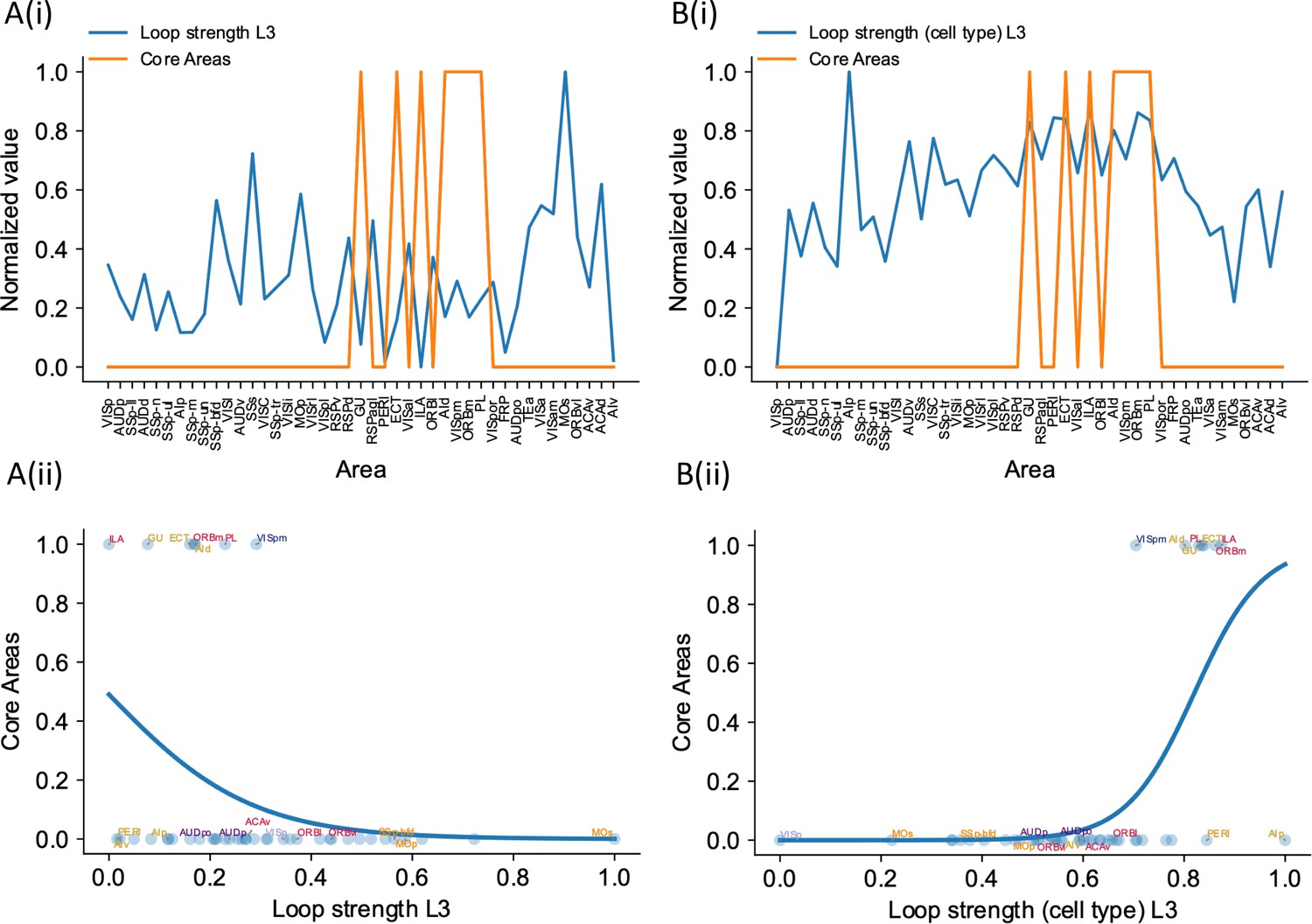
Loop strengths (length 3 loops or L3) is calculated using similar method as loop strengths (length 2 loops). The only difference is we considered loops with length 3 (e.g., A1->A2->A3->A1). The analysis is the same as in Figure 7, where we compared cell type-specific loop strengths (length 2 loops) and raw loop strengths. (A(i)) Loop strength (blue) is plotted alongside core areas (orange), a binary variable that takes the value 1 if the area is indeed a core area, 0 otherwise. Loop strength is normalized to a range of (0, 1) for better comparison. (A(ii)) A high loop strength value does not imply that an area is a core area. (B(i)) Same as (A), but for cell type-specific loop strength. (B(ii)) High cell type-specific loop measures predicts that an area is a core area (prediction accuracy = 0.95). Same as (A), but for cell type-specific loop strength.
Figure 8—figure supplement 2
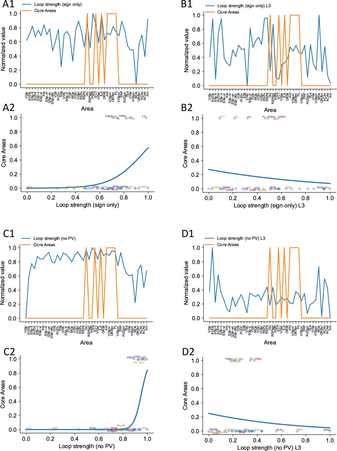
Sign-only loop strengths or noPV loop strengths are not performing well at predicting firing rate patterns.
(A1) Relationship between core areas (orange) and length 2 (sign only) loop strength. Areas are sorted according to their hierarchy. Whether an area is a core area is represented in either 0 or 1. (A2) High loop strength is a good predictor of whether an area is a core area. Blue curve shows the logistic regression analysis used to differentiate the core areas versus non-core areas (prediction accuracy = 0.83). (B1) and (B2) Same as (A1) and (A2), but with length 3 sign-only loop strength. Length 3 sign-only loop strength does not show a positive relationship with core areas (prediction accuracy = 0.83) (C1) and (C2) Same as (A1) and (A2), except for comparing whether an area is a core area (orange) and length 2 noPV loop strength. Length 2 noPV loop strength predicts the core areas. prediction accuracy = 0.90 (D1) and (D2) Same as (A1) and (A2), except for comparing whether an area is a core area (orange) and length 3 noPV loop strength. Length 3 noPV loop strength does not show a positive relationship with core areas. prediction accuracy = 0.83.
Figure 9
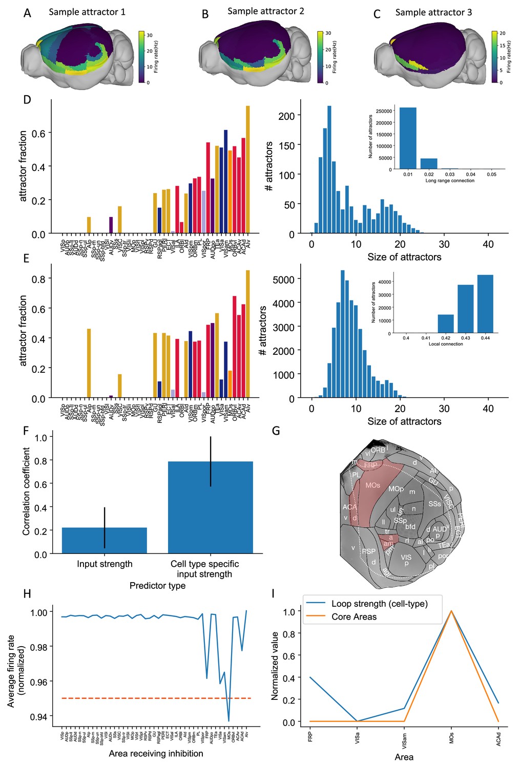
Multiple attractors coexist in the mouse working memory network.
(A–C) Example attractor patterns with a fixed parameter set. Each attractor pattern can be reached via different external input patterns applied to the brain network. Delay activity is shown on a 3D brain surface. Color represents the firing rate of each area. (D, E) The distribution of attractor fractions (left) and number of attractors as a function of size (right) for different parameter combinations are shown. Attractor fraction of an area is the ratio between the number of attractors that include the area and the total number of identified attractors. In (D), local excitatory strengths are fixed (=0.44 nA) while long-range connection strengths vary in the range = 0.01–0.05 nA. Left and right panels of (D) show one specific parameter = 0.03 nA. Inset panel of (D) shows the number of attractors under different long-range connection strengths while is fixed at 0.44 nA. In (E), long-range connection strengths are fixed (=0.02 nA) while local excitatory strengths varies in the range = 0.4–0.44 nA. Left and right panels of (E) show one specific parameter = 0.43 nA. Inset panel of (E) shows the number of attractors under different local excitatory strengths, while is fixed at 0.02 nA. (F) Prediction of the delay-period firing rate using input strength and cell type-specific input strength for each attractor state identified under = 0.04 nA and = 0.44 nA. A total of 143 distinct attractors were identified and the average correlation coefficient using cell type-specific input strength is better than that using input strength. (G) A example attractor state identified under the parameter regime = 0.03 nA and = 0.44 nA. The five areas with persistent activity are shown in red. (H) Effect of single area inhibition analysis for the attractor state in (G). For a regime where five areas exhibit persistent activity during the delay period, inactivation of the premotor area MOs yields a strong inhibition effect (<0.95 orange dashed line) and is therefore a core area for the attractor state in (G). (I) Cell type-specific loop strength (blue) is plotted alongside core areas (orange) for the attractor state in (G). Only five areas with persistent activity are used to calculate the loop strength. Loop strength is normalized to be within the range of 0 and 1. High cell type-specific loop measures predict that an area is a Core area (prediction accuracy is 100% correct). The number of areas is limited, so prediction accuracy is very high.
© 2019, Harris et al. Panel G is modified from Figure 1b of Harris et al., 2019 with permission. It is not covered by the CC-BY 4.0 licence and further reproduction of this panel would need permission from the copyright holder.
Tables
Table 1
Supplementary experimental evidence.
The listed literature include experiments that provide supporting evidence for working memory activity in cortical and subcortical brain areas in the mouse or rat. These studies show either that a given area is involved in working memory tasks and/or exhibit delay period activity. Area name corresponds to what has been reported in the literature. Some areas do not correspond exactly to the names from the Allen common coordinate framework.
| Area | Supporting literature |
|---|---|
| ALM (MOs) (anterior lateral motor cortex) | Guo et al., 2014; Li et al., 2016; Guo et al., 2017; Gilad et al., 2018; Inagaki et al., 2019; Wu et al., 2020; Voitov and Mrsic-Flogel, 2022; Kopec et al., 2015; Erlich et al., 2011; Gao et al., 2018, |
| mPFC (PL/ILA) (medial prefrontal cortex) | Liu et al., 2014; Schmitt et al., 2017, |
| Bolkan et al., 2017 | |
| OFC (orbitofrontal cortex) | Wu et al., 2020 |
| PPC (VISa, VISam) (posterior parietal cortex) | Voitov and Mrsic-Flogel, 2022; Harvey et al., 2012 |
| AIa (AId, AIv) | Zhu et al., 2020 |
| Area p (VISpl) | Gilad et al., 2018 |
| Dorsal cortex | Pinto et al., 2019 |
| Entorhinal (in vitro persistent activity) | Egorov et al., 2002 |
| Piriform | Zhang et al., 2019; Wu et al., 2020 |
| VM/VAL (ventromedial nucleus, ventroanterior-lateral complex) | Guo et al., 2017 |
| MD (mediodorsal nucleus) | Schmitt et al., 2017; Bolkan et al., 2017 |
| Superior colliculus | Kopec et al., 2015 |
| Cerebellar nucleus | Gao et al., 2018 |
Table 2
Parameters for numerical simulations.
| Parameter | Description | Task/figure | Value |
|---|---|---|---|
| Cortical circuit parameters | |||
| NMDA synapse time constant | All figures | 60 ms | |
| GABA synapse time constant | All figures | 5 ms | |
| AMPA synapse time constant | All figures | 2 ms | |
| Neuron time constant | All figures | 2 ms | |
| Noise time constant | All figures | 2 ms | |
| Parameters in excitatory F–I curve | All figures | 140 Hz/nA, 54 Hz, 308ms | |
| Parameters in inhibitory F–I curve | All figures | 4, 615 Hz/nA, 177 Hz, 5.5 Hz | |
| Parameters in NMDA excitatory synaptic equations | All figures | 1.282 | |
| Parameters in GABA synaptic equations | All figures | 2 | |
| Parameters in AMPA excitatory synaptic equations | All figures | 2 | |
| Local self-excitatory connections | Figures 1—8 | 0.4 nA | |
| Local cross-population excitatory connections | All figures | 10.7 pA | |
| Local E to I connections | All figures | 0.2656 nA | |
| Local I to E connection strength | All figures | 0.192 nA, 0.83 | |
| Local I to I connection strength | All figures | 0.105 nA, 0.714 | |
| Background current for excitatory neurons | All figures | 0.305 nA | |
| Background current for inhibitory neurons | All figures | 0.26 nA | |
| Standard deviation of excitatory noise current | All figures | 5 pA | |
| Standard deviation of inhibitory noise current | All figures | 0 pA | |
| Initial firing rate for excitatory neurons | All figures | 5 Hz | |
| Initial firing rate for inhibitory neurons | All figures | 5.5 Hz | |
| Long-range E to E connection strength | Figures 1—4, 6–7 | 0.1 nA | |
| Long-range E to I connection strength | Figures 1—4, 6–7 | 0.167 nA | |
| Parameters in mij | All figures | 2.42 | |
| Parameters for scaling the connectivity matrix | All figures | 0.3 | |
| Parameters for estimation of hierarchy | All figures | 1.33,-0.22 | |
| External stimulus strength | All figures | 0.5 nA | |
| External input to inhibitory neurons | All figures | 5 nA | |
| Stimulus start time | All figures | 2 s | |
| Stimulus end time | All figures | 2.5 s | |
| Simulation time for each trial | All figures | 10 s | |
| Simulation time step | All figures | 0.5ms | |
| Thalamocortical network | |||
| Long-range E to E connection strength | Figure 5 | 0.01 nA | |
| Long-range E to I connection strength | Figure 5 | 0.0167 nA | |
| Corticothalamic connections strength | Figure 5 | 0.32 nA | |
| Thalamocortical connections to excitatory neurons | Figure 5 | 0.6 nA | |
| Thalamocortical connections to inhibitory neurons | Figure 5 | 1.38 nA | |
| Simulation of multiple attractors | |||
| Long-range E to E connection strength | Figure 9 | 0.01, 0.02, 0.03, 0.04, 0.05 nA | |
| Long-range E to I connection strength | Figure 9 | 0.0167, 0.033, 0.05, 0.066, 0.083 nA | |
| Local self-excitatory connections | Figure 9 | 0.4, 0.41, 0.2, 0.43, 0.44 nA |
Additional files
Download links
A two-part list of links to download the article, or parts of the article, in various formats.
Downloads (link to download the article as PDF)
Open citations (links to open the citations from this article in various online reference manager services)
Cite this article (links to download the citations from this article in formats compatible with various reference manager tools)
Cell type-specific connectome predicts distributed working memory activity in the mouse brain
eLife 13:e85442.
https://doi.org/10.7554/eLife.85442


