Large-scale neural dynamics in a shared low-dimensional state space reflect cognitive and attentional dynamics
- Department of Psychology, University of Chicago, United States
- Department of Biomedical Engineering, Sungkyunkwan University, Republic of Korea
- Center for Neuroscience Imaging Research, Republic of Korea
- Department of Intelligent Precision Healthcare Convergence, Sungkyunkwan University, Republic of Korea
- Neuroscience Institute, University of Chicago, United States
Figures
Figure 1 with 8 supplements
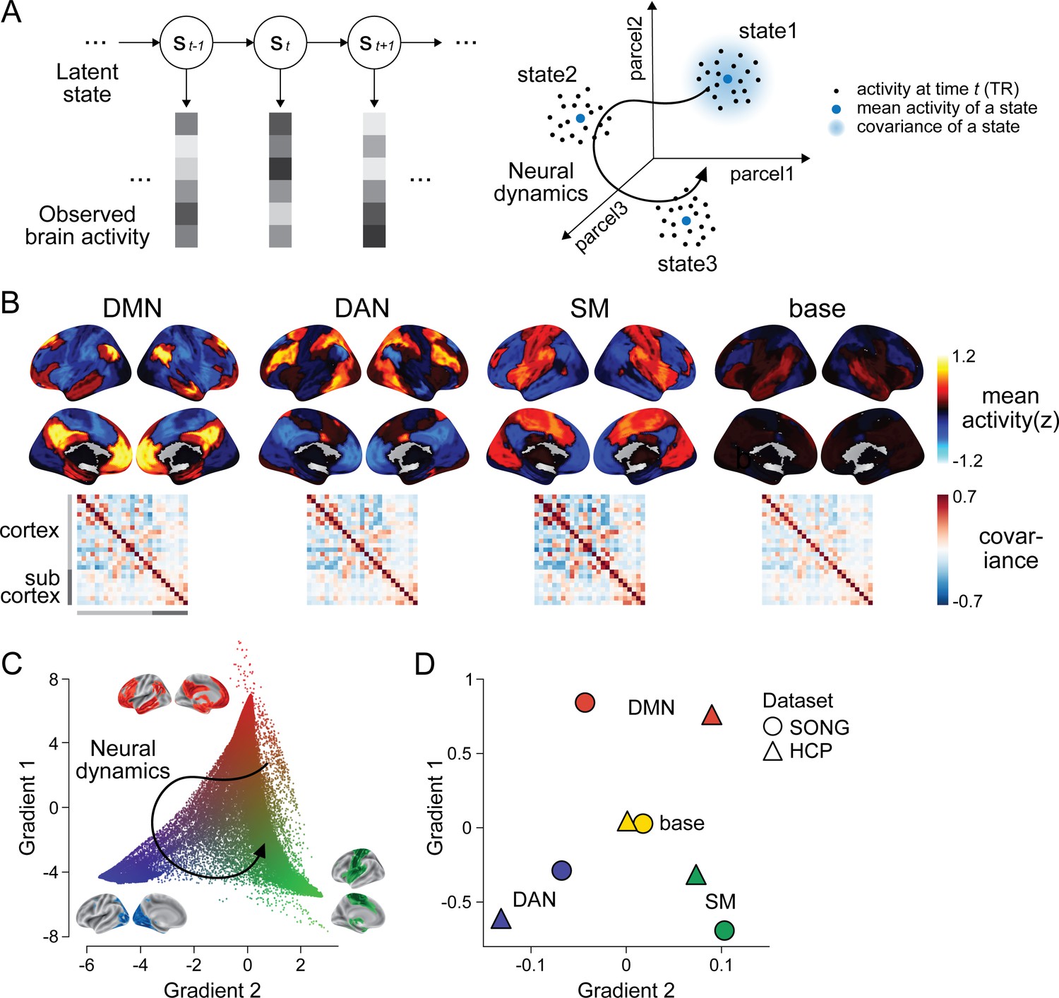
Latent state space of the large-scale neural dynamics.
(A) Schematic illustration of the hidden Markov model (HMM) inference. (Left) The HMM infers a discrete latent state sequence from the observed 25-parcel fMRI time series. (Right) The fMRI time course can be visualized as a trajectory within a 25-dimensional space, where black dots indicate activity at each moment in time. The HMM probabilistically infers discrete latent clusters within the space, such that each state can be characterized by the mean activity (blue dots) and covariance (blue shaded area) of the 25 parcels. (A) has been adapted from Figure 1A from Cornblath et al., 2020. (B) Four latent states inferred by the HMM fits to the SONG dataset. Mean activity (top) and pairwise covariance (bottom) of the 25 parcels’ time series is shown for each state. See Figure 1—figure supplement 6 for replication with the Human Connectome Project (HCP) dataset. (C) Conceptualizing low-dimensional gradients of the functional brain connectome as a latent manifold of large-scale neural dynamics. Each dot corresponds to a cortical or subcortical voxel situated in gradient space. The colors of the brain surfaces (inset) indicate voxels with positive or negative gradient values with respect to the nearby axes. Data and visualizations are adopted from Margulies et al., 2016. (D) Latent neural states situated in gradient space. Positions in space reflect the mean element-wise product of the gradient values of the 25 parcels and mean activity patterns of each HMM state inferred from the SONG (circles) and HCP (triangles) datasets.
Figure 1—figure supplement 1
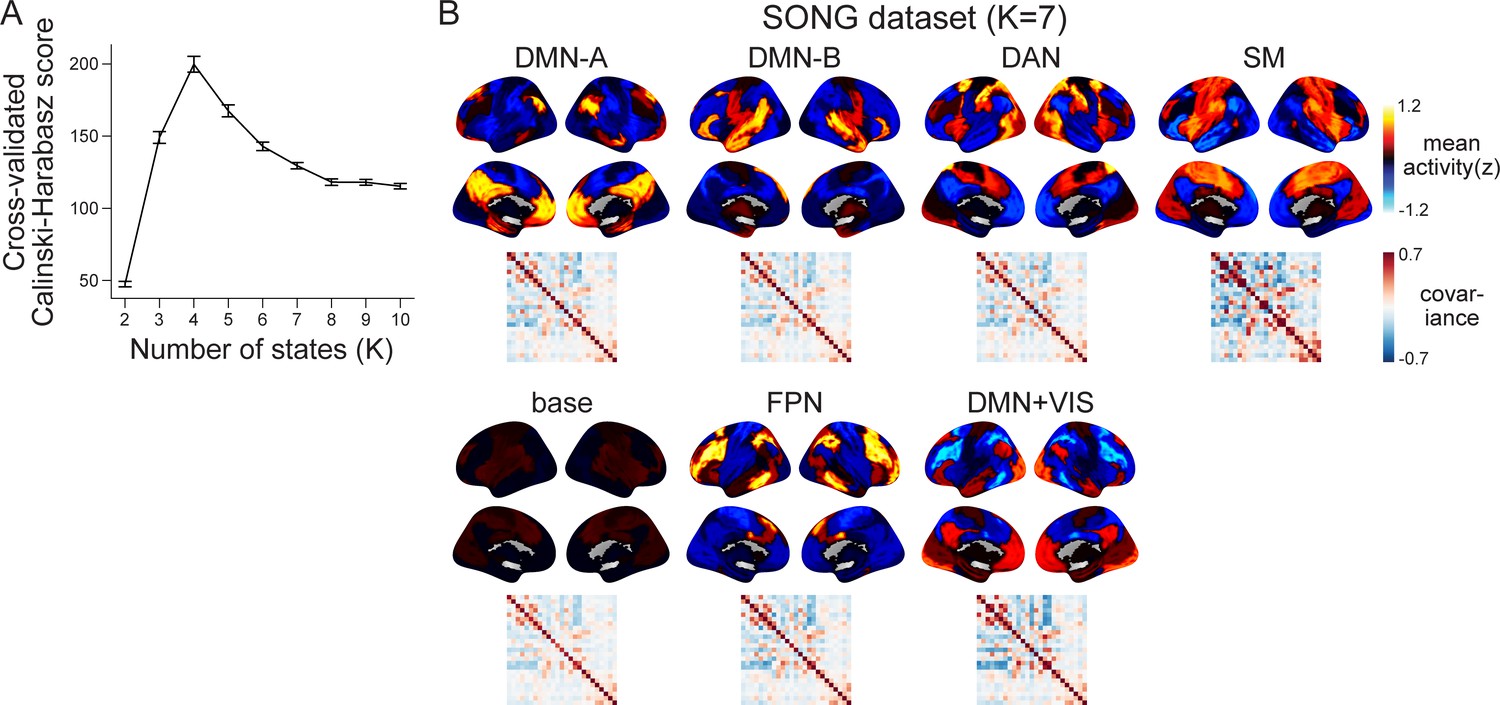
The choice of the number of states (K) in latent state inference.
(A) To determine a value of K that optimizes hidden Markov model (HMM) state inference from the SONG dataset, we iteratively calculated the Calinski–Harabasz scores using leave-one-subject-out cross-validation with K ranging from 2 to 10. Specifically, the HMM was trained on data from all participants but one to estimate parameters: emission and transition probabilities. The model was then applied to decode the latent state sequence of the held-out participant. With the held-out participant’s fMRI time series, the BOLD pattern similarity of the within- versus across- latent states were compared using the Calinski–Harabasz score, such that higher score indicates higher within-state cluster cohesion compared to the across-state dispersion (Calinski and Harabasz, 1974; Gao et al., 2021; Song et al., 2021b). The line indicates the mean of the cross-validated Calinski–Harabasz scores and the error bars indicate SEM. (B) HMM latent neural states inferred from the SONG dataset using a different choice of K (K = 7). When more states were inferred, we observed subdivisions of and additions to the four neural states in Figure 1B. The dorsal attention network (DAN), somatosensory motor (SM), and base states appeared with similar activity patterns (r = 0.678, 0.923, and 0.445, respectively). The default mode network (DMN) state was subdivided into two DMN states. The DMN-A corresponded to the DMN core and the medial temporal subsystem. The DMN-B corresponded to the dorsal medial subsystem (Andrews-Hanna et al., 2014). Two additional neural states were inferred: one which exhibited the highest activity at the frontoparietal network (FPN) and the other showing activity in both the DMN and visual network (VIS).
Figure 1—figure supplement 2
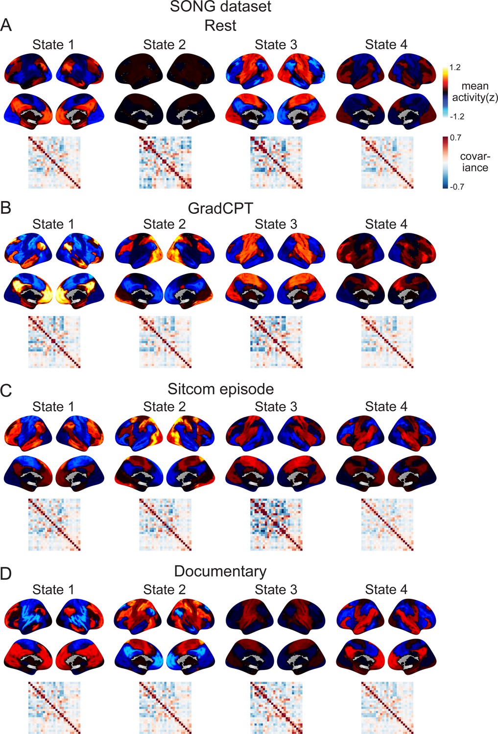
Latent state inference conducted separately to each condition of the SONG dataset.
(A) Rest includes the two resting-state runs (600 TR × 2 for every 27 participants), (B) GradCPT includes the two gradCPT runs with face (511 TR) and scene (443 TR) images, (C) Sitcom episode includes the two sitcom-episode-watching runs (episode 1: 1486 TR; episode 2: 1465 TR), and (D) Documentary corresponds to the single documentary-watching run (1281 TR). The states are ordered based on the activation pattern similarity to the default mode network (DMN), dorsal attention network (DAN), somatosensory motor (SM), and base states inferred from the full dataset (Figure 1B). The pattern similarities are as follows in the order of DMN, DAN, SM, and base states: Rest: r = 0.801, 0.332, 0.722, 0.369; GradCPT: r = 0.956, 0.747, 0.928, 0.276; Sitcom ep: r = 0.486, 0.600, 0.737, 0.882; Documentary: r = 0.526, 0.847, 0.747, 0.663.
Figure 1—figure supplement 3
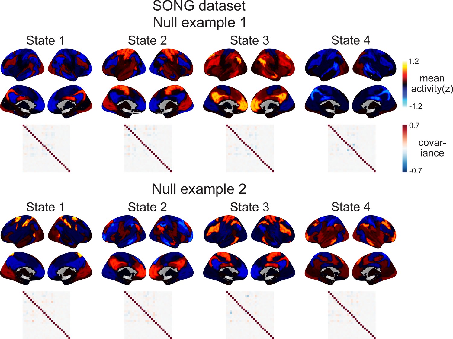
Examples of the null latent states derived from the hidden Markov models (HMMs) conducted on the surrogate fMRI time series of the SONG dataset (1000 iterations).
The 25 parcel time courses from each fMRI run and participant were circular-shifted, separately for each parcel, which disrupts the covariance across parcels while retaining the temporal characteristics of each individual parcel. Compared to the latent states derived from the actual fMRI time series (Figure 1B), these null states did not show systematic activity patterns and exhibited weaker covariance strengths. In Figure 1B, the somatosensory motor (SM) state exhibited the highest covariance strength (SONG: 52.570; Human Connectome Project [HCP]: 58.196), followed by comparable default mode network (DMN) state (SONG: 37.277; HCP: 28.353) and dorsal attention network (DAN) state (SONG: 37.303; HCP: 29.525), whereas the base state exhibited the lowest covariance strength (SONG: 27.603; HCP: 25.426). On the contrary, the mean covariance strengths of the four surrogate covariance matrices were in the range of 3.215–4.432 for SONG and 0.986–2.204 for HCP datasets over 1000 iterations.
Figure 1—figure supplement 4
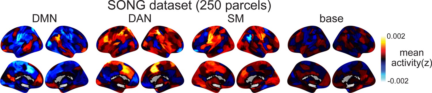
Latent state inference using a different whole-brain parcellation scheme.
In the main text, we chose a fairly low-dimensional parcellation scheme (17 cortical and 8 subcortical) because the hidden Markov model (HMM) produces a poorer fit when the dimensionality of the time series increases. The reason is that the number of parameters that need to be inferred for emission probability, increase exponentially with the increase in the number of parcel dimension . Here, we test the robustness of the four latent states by using 200 cortical and 50 subcortical parcels, but applied dimensionality reduction to these 250 parcel time series prior to using them as inputs to the HMM. The matrices were randomly projected to 25-dimensional time series matrices by multiplying the time-by-250 matrix with the randomly generated 250-by-25 matrices. Random projection is a validated dimensionality reduction tool (Bingham and Mannila, 2001) that does not impose any constraints on how the latent dimensions should be (e.g., the principal component analysis should find latent dimensions that maximize explained variance and are orthogonal to one another). The HMM fit was conducted 500 times. For each iteration, after the HMM fit, we inverse-projected 25-dimensional mean activation patterns to 250 dimensions. The decoded latent state sequence of each iteration was compared to the decoded state sequence of the 25-parcel time series that we report in the manuscript. By finding the latent state sequence that shows the highest sequence similarity (mean 40.7 ± 3.45%, given a chance of 25%), we reordered the estimated mean activations and averaged across 500 iterations. The Pearson’s correlations between these average activation patterns and the inferred latent states in Figure 1B are default mode network (DMN): 0.549; dorsal attention network (DAN): 0.406; somatosensory motor (SM): 0.487; and base: 0.178. Thus, we see similar states in the SONG dataset even when input time series do not come from canonical functional networks. The DMN, DAN, SM, and base states are not specific to the parcellation scheme presented in the main text.
Figure 1—figure supplement 5
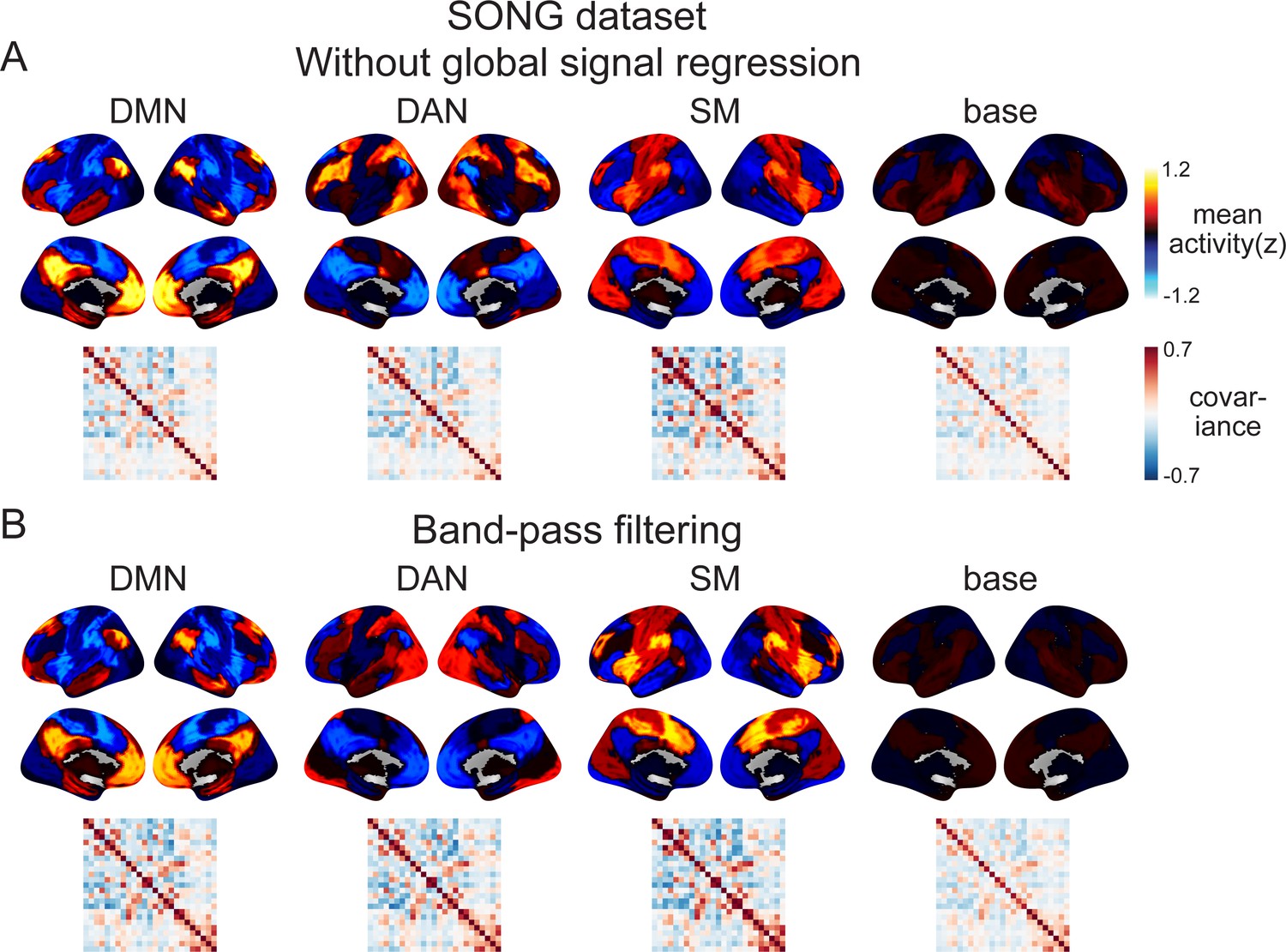
The inferred latent states and their dynamics are robust to the choice of the fMRI preprocessing approach.
(A) We conducted hidden Markov model (HMM) on preprocessed fMRI time series that did not undergo global signal regression. The output time series were highly similar with or without global signal regression, resulting in similar neural state dynamics (93.96% of the time points the same when assigned to the best-matching state, given a chance of 25%) and similar activity patterns of the four latent states (r = 0.999, 1.0, 0.997, and 0.997, respectively). (B) We conducted HMM on the preprocessed fMRI time series that were temporally band-pass filtered (0.009 < f < 0.08 Hz) rather than high-pass filtered (f > 0.009 Hz). The inferred neural states had similar activity patterns (r = 0.961, 0.709, 0.883, and 0.757), though their dynamics were not as similar as in (A) (28.59% of the time points the same). However, for all results reported in the article, we validated that the results were replicated in the band-pass filtered version of the analysis.
Figure 1—figure supplement 6
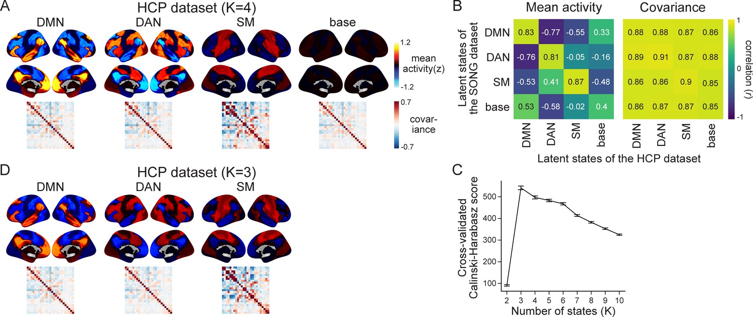
Latent state inference on the Human Connectome Project (HCP) dataset.
(A) Four latent states inferred by the hidden Markov model (HMM) fits to the HCP dataset. The figure complements Figure 1B. (B) Comparison of the latent states inferred from the SONG (Figure 1B) and HCP datasets. The default mode network (DMN), dorsal attention network (DAN), and somatosensory motor (SM) states showed similar mean activity patterns. We refrained from making interpretations about the base state’s activity patterns because the mean activity of most of the parcels was close to z = 0. The covariance patterns were similar throughout all pairwise neural states, although covariance strength values differed across neural states. To further validate the similarity of the SONG- and HCP-identified latent states, we trained the HMM on each dataset and applied it to decode the latent state sequence of the other dataset. When the SONG-trained HMM decoded the latent state sequence of the HCP dataset, 61.18% of the time points were the same as the latent state sequence identified from the HCP-trained HMM (with a chance of 25%). When the HCP-trained HMM decoded the latent state sequence of the SONG dataset, 61.67% of the time points were the same as the latent state sequence identified from the SONG-trained HMM. (C) Calinski–Harabasz score calculated from the HCP dataset (leave-one-subject-out cross-validation with K ranging from 2 to 10). (D) HMM latent states inferred from the HCP dataset using K = 3. The DMN, DAN, and SM states occurred for both the choice of K = 3 and K = 4 (activity pattern similarity: r = 0.981, 0.984, and 0.911, respectively).
Figure 1—figure supplement 7
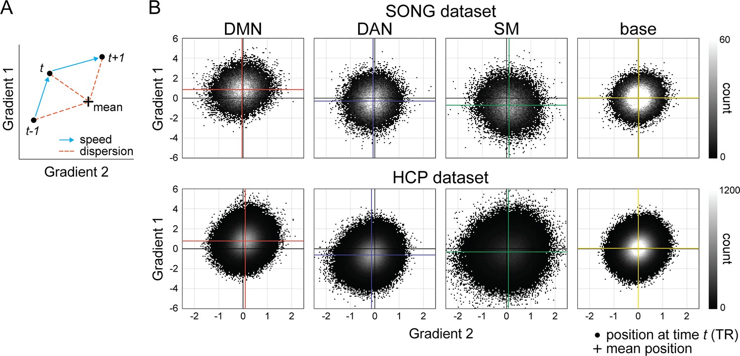
The position in predefined gradient space at every time point grouped by hidden Markov model (HMM) latent state.
(A) Schematic illustration of the timepoint distribution and the speed and dispersion measurements. Each black dot indicates 25-parcel BOLD activity patterns situated in the two-dimensional gradient space. Speed characterizes Euclidean distance between the gradient positions at time t-1 and t, such that fast speed indicates large Euclidean distance. Dispersion characterizes Euclidean distance between the gradient position at time t and the centroid (i.e., mean position of each latent state, indicated with a cross). (B) Activity at every time point (TR) of the SONG (top) and Human Connectome Project (HCP) (bottom) datasets situated in gradient space, categorized based on the latent state assignment at each moment. Positions in the space reflect the element-wise product of the gradient values and the z-normalized BOLD activity of the 25 parcels, which are stacked as a 2D histogram. The colored crosses indicate the means of the distribution in predefined gradient 1 and 2 axes. Mean speeds of the four states are: (SONG) default mode network (DMN): 0.715, dorsal attention network (DAN): 0.710, somatosensory motor (SM): 0.797, base: 0.672; (HCP) DMN: 0.568, DAN: 0.535, SM: 0.712, base: 0.554. Mean dispersions of the four states are: (SONG) DMN: 0.964, DAN: 1.0, SM: 1.139, base: 0.830; (HCP) DMN: 0.946, DAN: 0.835, SM: 1.257, base: 0.889. The Euclidean distances are calculated in the two-dimensional predefined gradient space, thus the relative units between the latent states are of importance. The SM state exhibited the fastest neural dynamics and the largest deviance from the mean, whereas the base state exhibited the slowest neural dynamics near the center of the mean.
Figure 1—figure supplement 8
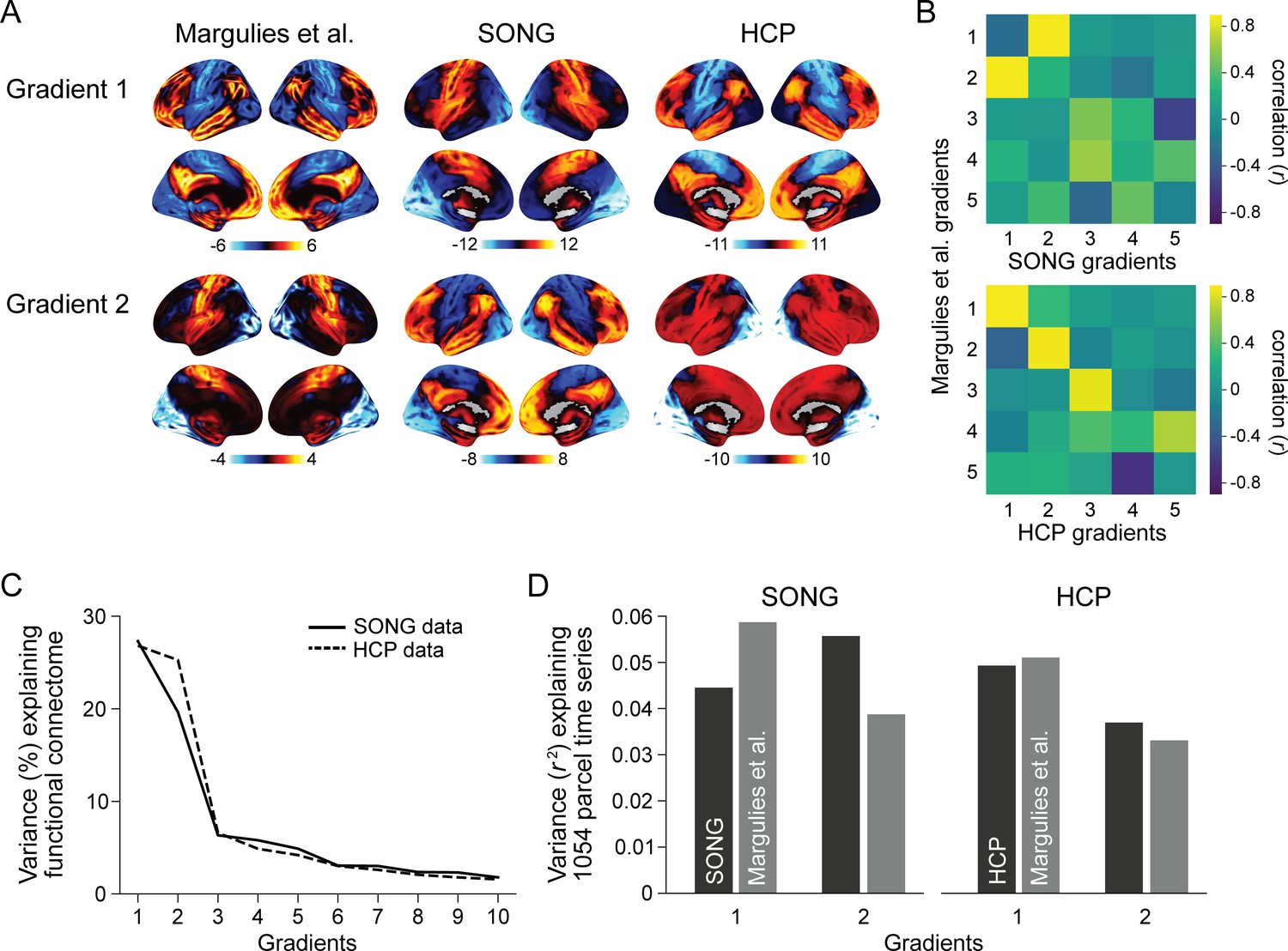
Comparisons between predefined and data-specific gradients.
(A) (Left) Visualization of the Margulies et al.’s (2016) first two gradient embeddings (left). The predefined gradients were downloaded from https://identifiers.org/neurovault.collection:1598. Visualization of the first two gradient embeddings defined from the SONG data (middle) and the Human Connectome Project (HCP) data (right). The gradients were computed from the mean 1054 ROI-by-ROI functional connectivity matrix of all participants in each dataset. The 1054 parcels include 1000 cortical ROIs of the Schaefer et al., 2018 atlas and 54 subcortical ROIs of Tian et al., 2020 atlas. (B) Pearson’s correlations between the top 5 Margulies et al., 2016 gradient embeddings and the SONG data (top) and HCP data (bottom) gradient embeddings. The gradient embeddings were estimated from 1054 ROIs. (C) Variance of the SONG data participants’ average functional connectivity explained by the SONG-specific gradients (solid line). Variance of the HCP data participants’ average functional connectivity explained by the HCP-specific gradients (dashed line). (D) (Left) Variance of the SONG data fMRI time series (1054 ROIs) explained by the first two SONG data gradients (black) and Margulies et al., 2016 gradients (gray). (Right) Variance of the HCP data fMRI time series explained by the first two HCP data gradients (black) and Margulies et al., 2016 gradients (gray). The explained variance was calculated by the mean of squared Pearson’s correlations () between the 1054 ROI fMRI time series and the gradient-projected time series.
Figure 2 with 4 supplements

Neural state transitions.
(A) Changes in cofluctuation of the parcel pairs, time-aligned to hidden Markov model (HMM)-derived neural state transitions. State transitions occur between time t-1 and t. Purple lines indicate the mean cofluctuation of cortico-cortical (left), cortico-subcortical (middle), and subcortico-subcortical (right) parcel pairs across fMRI runs and participants, and the thick black line indicates the mean of these pairs. The shaded gray area indicates the range of the null distribution (mean ± 1.96 × standard deviation), in which the moments of state transitions were randomly shuffled (asterisks indicate FDR-p<0.05). (B) Transition matrix indicating the first-order Markovian transition probability from one state (row) to the next (column), averaged across all participants’ all fMRI runs. The values indicate transition probabilities, such that values in each row sums to 1. The colors indicate differences from the mean of the null distribution where the HMMs were conducted on the circular-shifted time series. (C) Mean degrees of global cofluctuation at moments of latent neural state occurrence. The measurements at each time point were averaged within participant based on latent state identification, and then averaged across participants. The bar graph indicates the mean of all participants’ all fMRI runs. The error bars indicate standard error of the mean (SEM). Gray dots indicate individual data points (7 runs of 27 participants). The shaded gray area indicates the range of the null distribution, in which the analyses were conducted on the circular-shifted latent state sequence. See Figure 2—figure supplement 1 for replication with the Human Connectome Project (HCP) dataset.
Figure 2—figure supplement 1
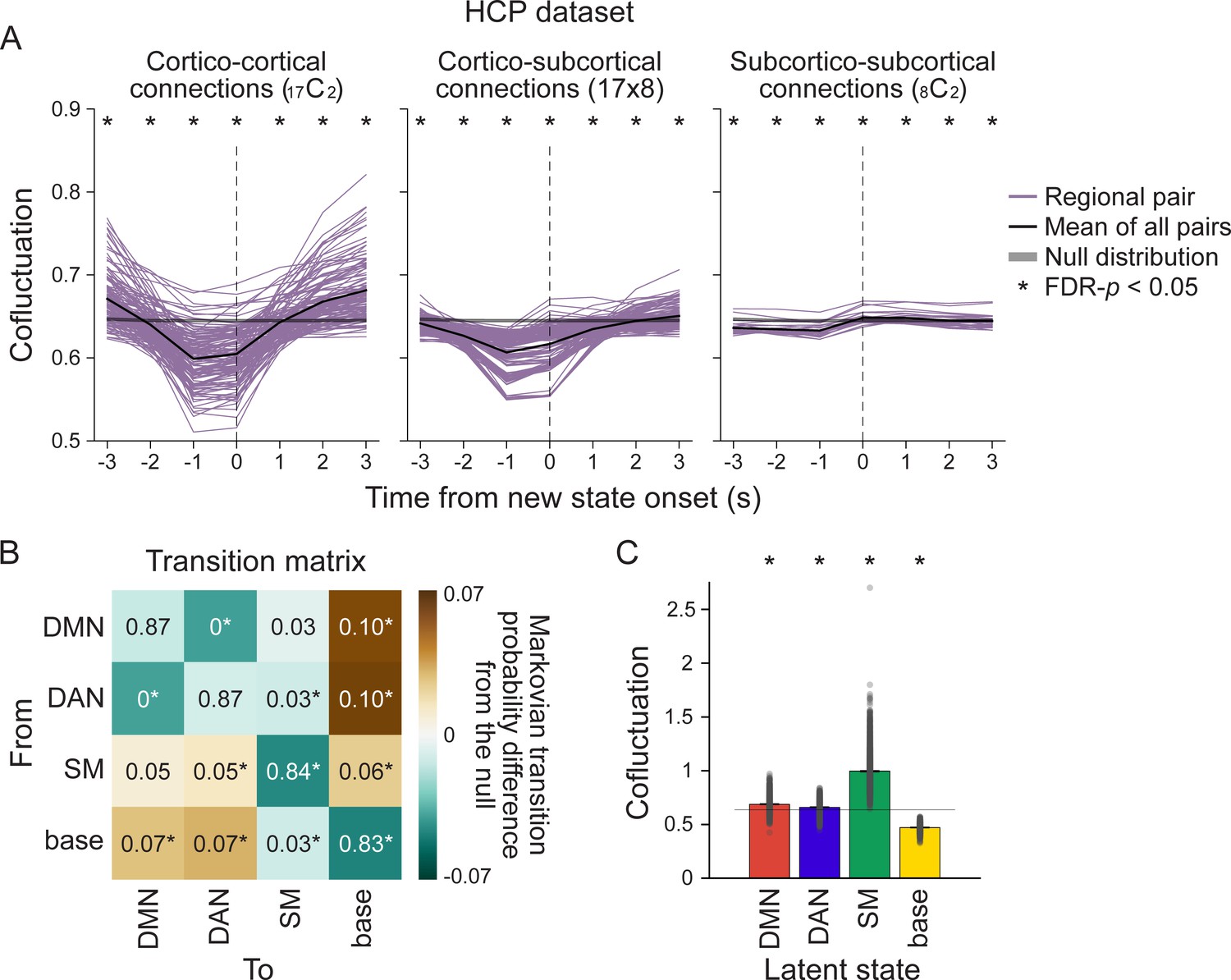
Neural state transitions of the Human Connectome Project (HCP) dataset.
Figure 2—figure supplement 2
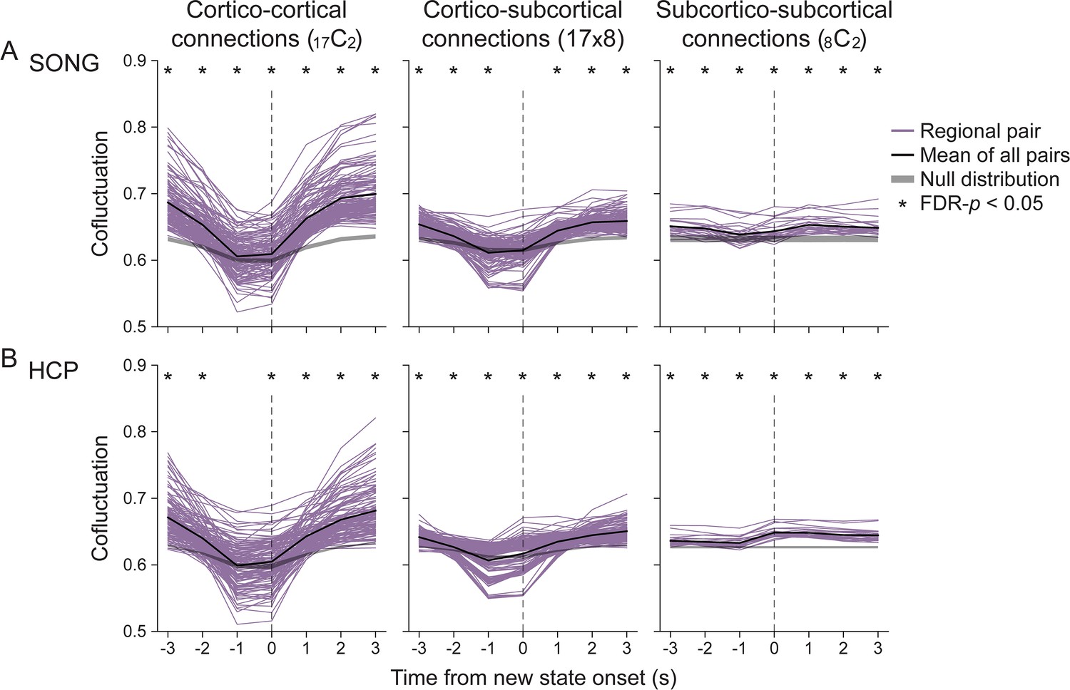
Cofluctuations of all pairs of 25 parcels of the (A) SONG and (B) Human Connectome Project (HCP) datasets, time-aligned to the hidden Markov model (HMM)-derived neural state transitions, compared to a null distribution that was generated differently than Figure 2A.
Instead of shuffling the moments of neural state transitions (Figure 2A), we circular-shifted the parcel time series prior to the HMM inference (1000 iterations, two-tailed non-parametric permutation tests, FDR-corrected for the number of time points). This way of creating null distribution allowed us to ask whether the HMM, by the nature of the model, detects state transitions based on transient decrease in the global synchrony. We observed a decrease in cofluctuation between cortico-cortical and cortico-subcortical regions prior to null state onset (difference between the mean cofluctuation at time t+3 and t-1 aligned to new state onset, bootstrapped p-values<0.001). However, this decrease was less dramatic than that observed in the actual fMRI time series (two-tailed non-parametric permutation tests, FDR-p-values<0.002, corrected for the three pair types). Thus, decreases in cofluctuation prior to state transitions are not simply a byproduct of the computational model.
Figure 2—figure supplement 3
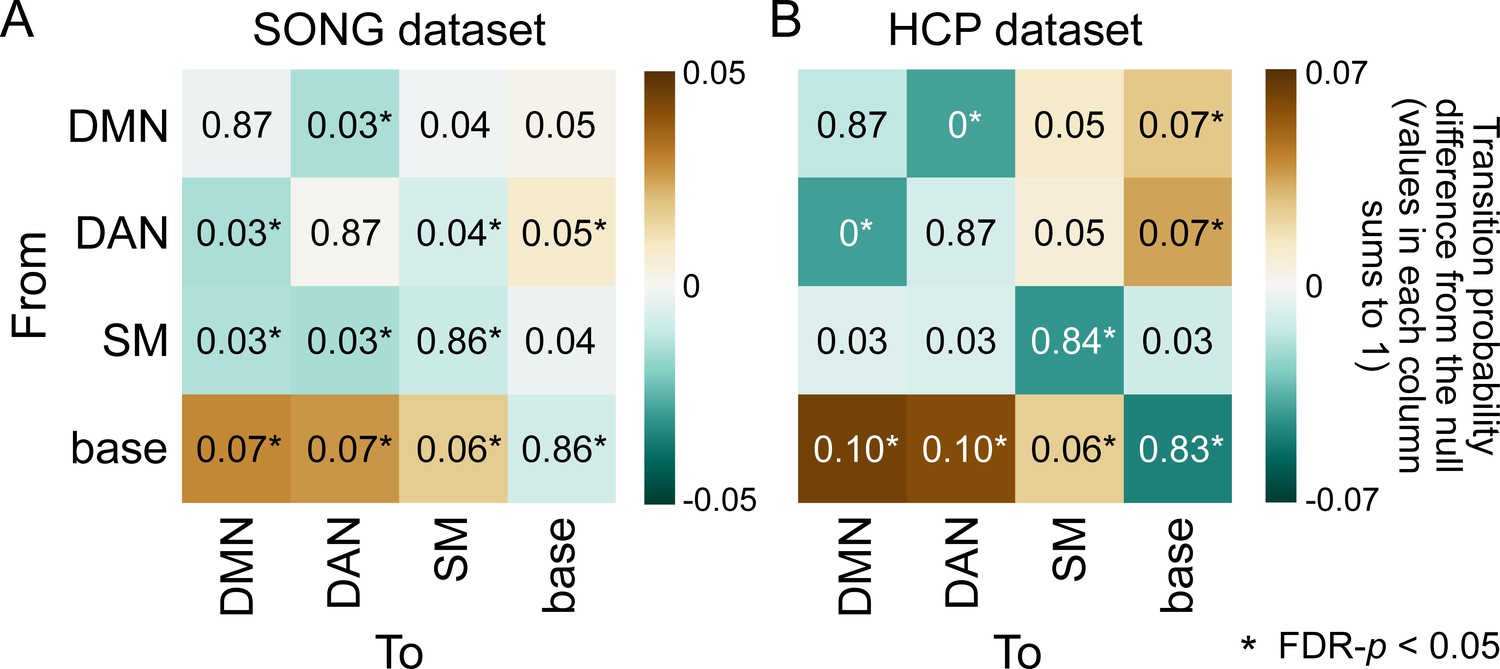
Transition matrix of the (A) SONG and (B) Human Connectome Project (HCP) datasets indicating transition probability from one state (row) to the next (column), such that values in each column sums to 1.
Complementing Figure 2B, which indicates the probability of transitioning to a certain brain state from each of the states (values in each row sums to 1), this figure indicates the probability of transitioning from each brain state. The colors indicate differences from the mean of the null distribution where the hidden Markov models (HMMs) were conducted on the circular-shifted time series (asterisks indicate FDR-p<0.05).
Figure 2—figure supplement 4
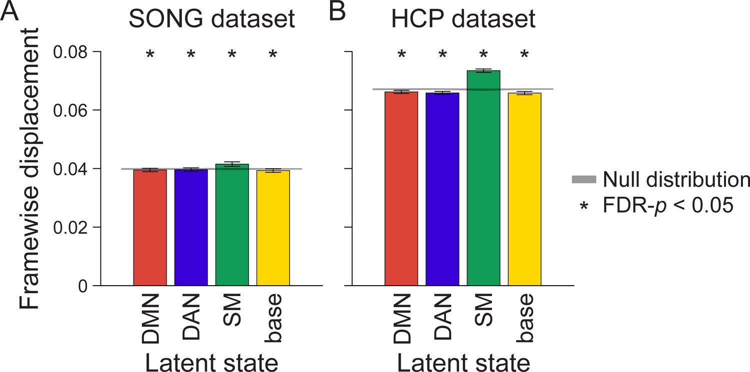
Mean head motion (framewise displacement [FD]) at moments of latent neural state occurrence in the (A) SONG and (B) Human Connectome Project (HCP) datasets.
FD measured at each time point was averaged within a participant based on the latent state identification, and then averaged across participants. The bar graph indicates the mean of FD from all fMRI runs and participants. The shaded gray area indicates the range of the null distribution (mean ± 1.96 × standard deviation), in which the analyses were conducted on the circular-shifted latent state sequence. FD was measured after motion correction. Higher FD was observed at TRs assigned to the somatosensory motor (SM) state than at TRs assigned to other states (paired t-tests, SONG: t(187) > 4, HCP: t(3091) > 22, both FDR-p-values<0.001, corrected for the number of pairwise states), but FD at moments of default mode network (DMN), dorsal attention network (DAN), and base states were comparable (SONG: t(187) < 1.5, HCP: t(3093) < 2, both FDR-p-values>0.15).
Figure 3 with 2 supplements
Latent neural state dynamics in the seven fMRI runs.
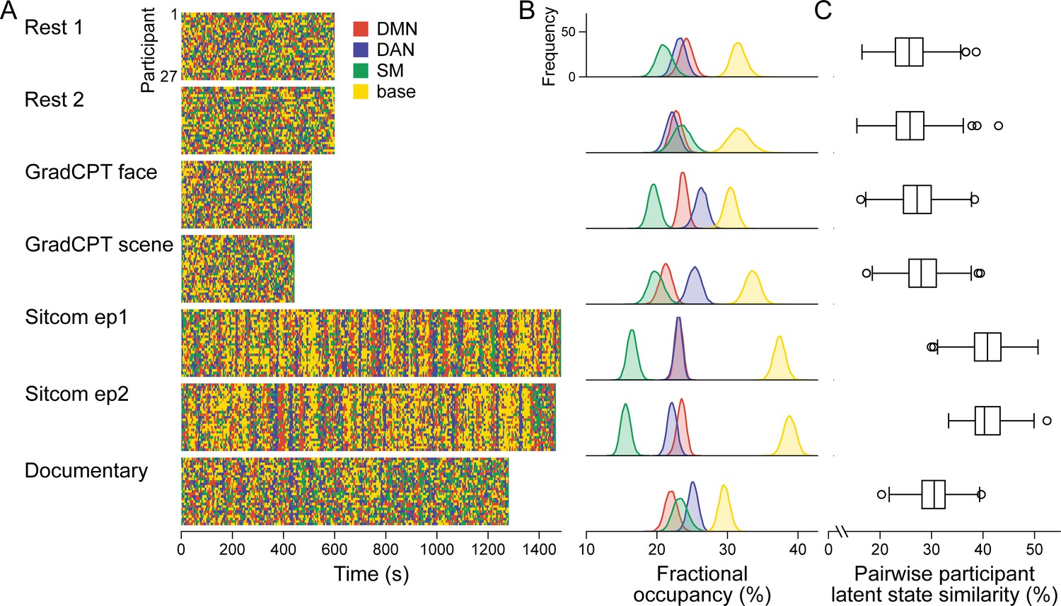
(A) Latent state dynamics inferred by the hidden Markov model (HMM) for all participants. Colors indicate the state that occurred at each time point. (B) Fractional occupancy of the neural states in each run. Fractional occupancy was calculated for each individual as the ratio of the number of time points at which a neural state occurred over the total number of time points in the run. Distributions indicate bootstrapped mean of the fractional occupancies of all participants. The chance level is at 25%. (C) Synchrony of latent state sequences across participants. For each pair of participants, sequence similarity was calculated as the ratio of the number of time points when the neural state was the same over the total number of time points in the run. Box and whisker plots show the median, quartiles, and range of the similarity distribution.
Figure 3—figure supplement 1
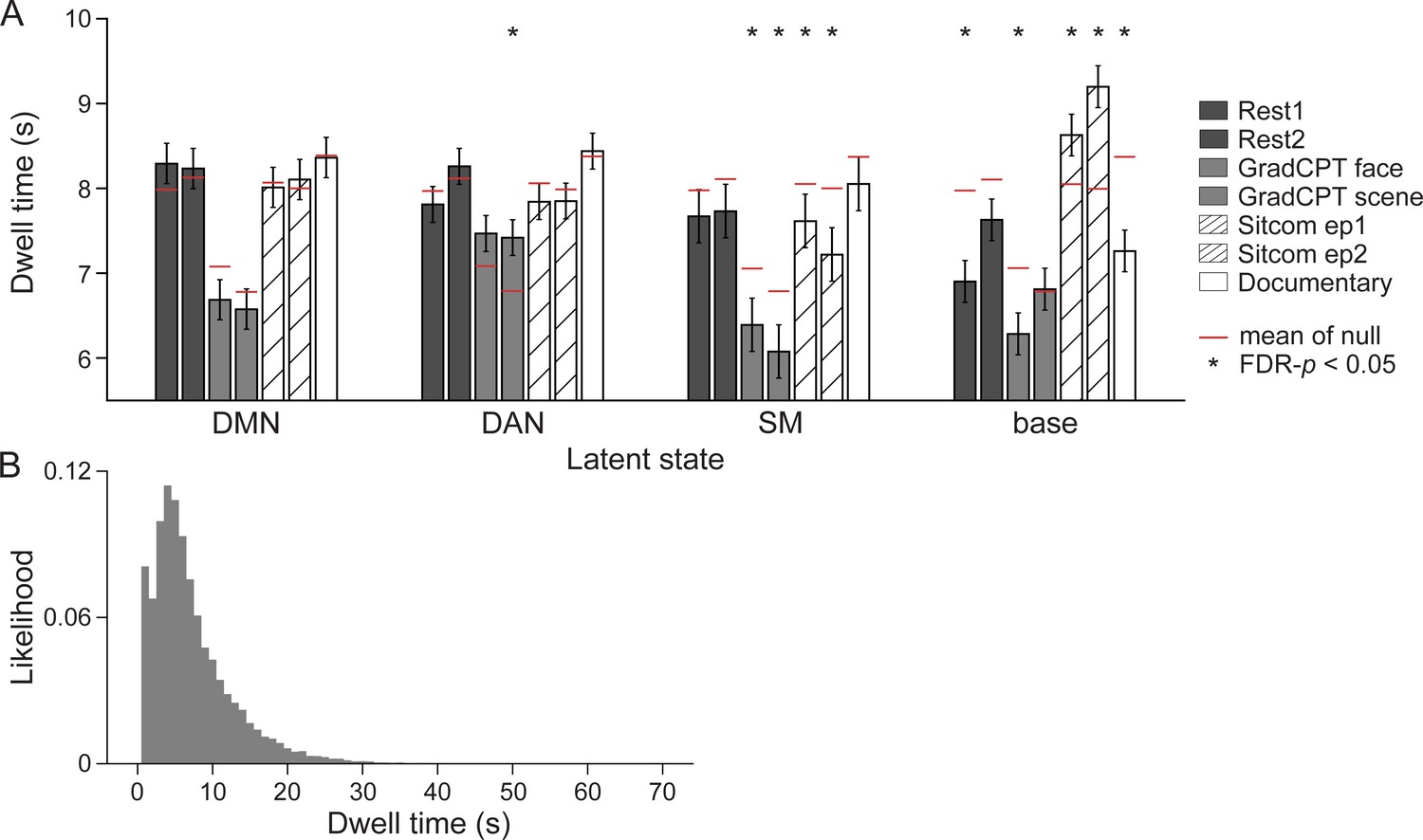
Dwell times of the latent neural states, measured as the duration (s) for which a neural state continuously persisted before transitioning to a different state.
(A) Mean dwell times of each latent state in every run of the SONG dataset. The mean dwell times of the null distribution, computed on the hidden Markov models (HMMs) conducted on the circular-shifted 25-parcel time series, are indicated in red. The significance of the two-tailed non-parametric permutation tests are indicated with asterisks (1000 iterations, FDR-p<0.05, corrected for 28 comparisons). For the resting-state runs, the dwell times of the base state were lower than the null dwell times. For the gradCPT runs, the dwell times of the dorsal attention network (DAN) state were higher whereas the dwell times of the somatosensory motor (SM) state were lower than the null. For the sitcom-episode-watching runs, the dwell times of the base state were higher, whereas the dwell times of the SM state were lower than the null. Lastly, for the documentary-watching run, base state dwell time was significantly lower than the null. (B) Histogram of all latent states’ dwell times. The dwell times of the state time course concatenated across 27 participants’ seven runs had a mean of 7.293 ± 5.680 s, median 6 s, ranging from 1 to 71 s.
Figure 3—figure supplement 2
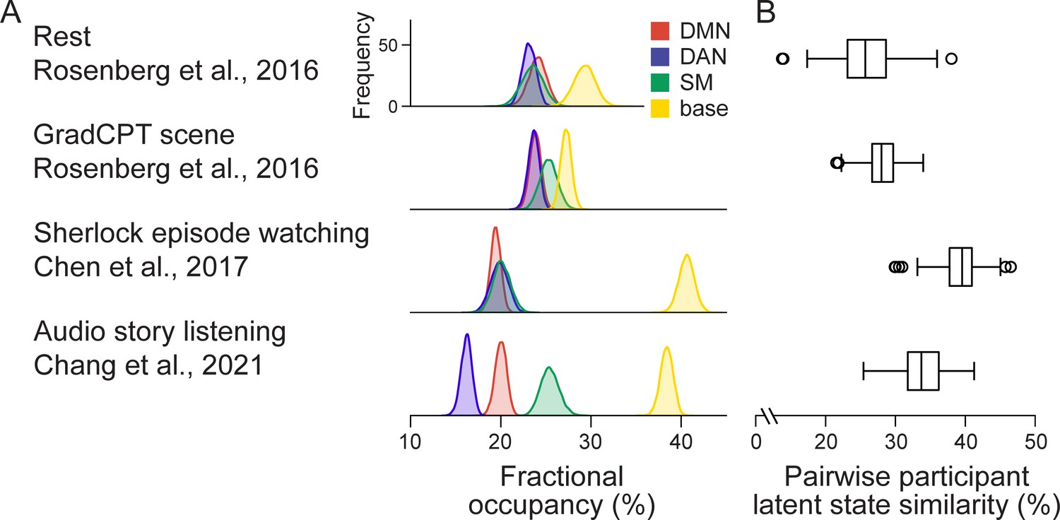
Inferred neural state dynamics of the external datasets from the hidden Markov model (HMM) trained on the SONG dataset.
To verify that the inferred neural states are not specific to these datasets, we applied the SONG-trained HMM (i.e., the inferred emission and transition probabilities) to decode latent sequences of the three independent datasets that targeted specific task contexts: the resting-state and gradCPT of Rosenberg et al., 2016 (N = 25), television episode watching of Chen et al., 2017 (N = 16), and story listening of Chang et al., 2021b (N = 25). (A) Fractional occupancy of the four latent states per dataset. (B) Latent state sequence similarity of all pairs of participants in each dataset. Intersubject synchrony of the latent state sequence was high during television episode watching (Chen et al., 2017) (39.24 ± 3.34%, FDR-p<0.001; comparable to synchrony during the SONG sitcom episodes) and story listening (Chang et al., 2021b) (33.84 ± 3.08%, FDR-p<0.001). In comparison, intersubject similarity during rest (Rosenberg et al., 2016) was near chance (25.84 ± 3.79%, though statistically significant FDR-p<0.001). The analysis follows Figure 3B and C.
Figure 4 with 2 supplements
Neural state occurrence and transitions at narrative event boundaries.
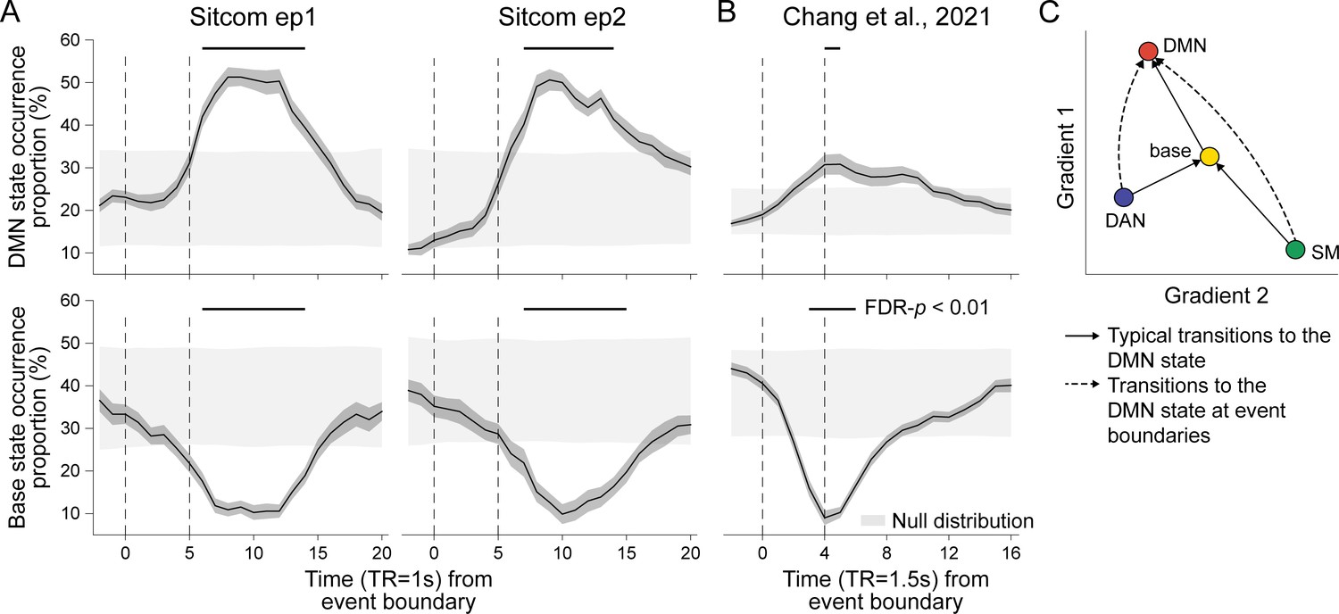
(A) The proportion of the default mode network (DMN) (top) and base state (bottom) occurrences time-aligned to narrative event boundaries of sitcom episodes 1 (left) and 2 (right). State occurrence at time points relative to the event boundaries per stimulus was computed within participant and then averaged across participants. The dark gray shaded areas around the thick black line indicate SEM. The dashed lines at t = 0 indicate moments of new event onset and the lines at t = 5 account for hemodynamic response delay of the fMRI. The light gray shaded areas show the range of the null distribution in which boundary indices were circular-shifted (mean ± 1.96 × standard deviation), and the black lines on top of the graphs indicate statistically significant moments compared to chance (FDR-p<0.01). (B) The proportion of the DMN (top) and base state (bottom) occurrence time-aligned to narrative event boundaries of audio narrative. Latent state dynamics were inferred based on the hidden Markov model (HMM) trained on the SONG dataset. Lines at t = 4 account for hemodynamic response delay. (C) Schematic transitions to the DMN state at narrative event boundaries (dashed lines) compared to the normal trajectory which passes through the base state (solid lines). See Figure 4—figure supplement 2 for results of statistical analysis.
Figure 4—figure supplement 1
Neural state occurrence and hippocampal BOLD activity time-aligned to narrative event boundaries.
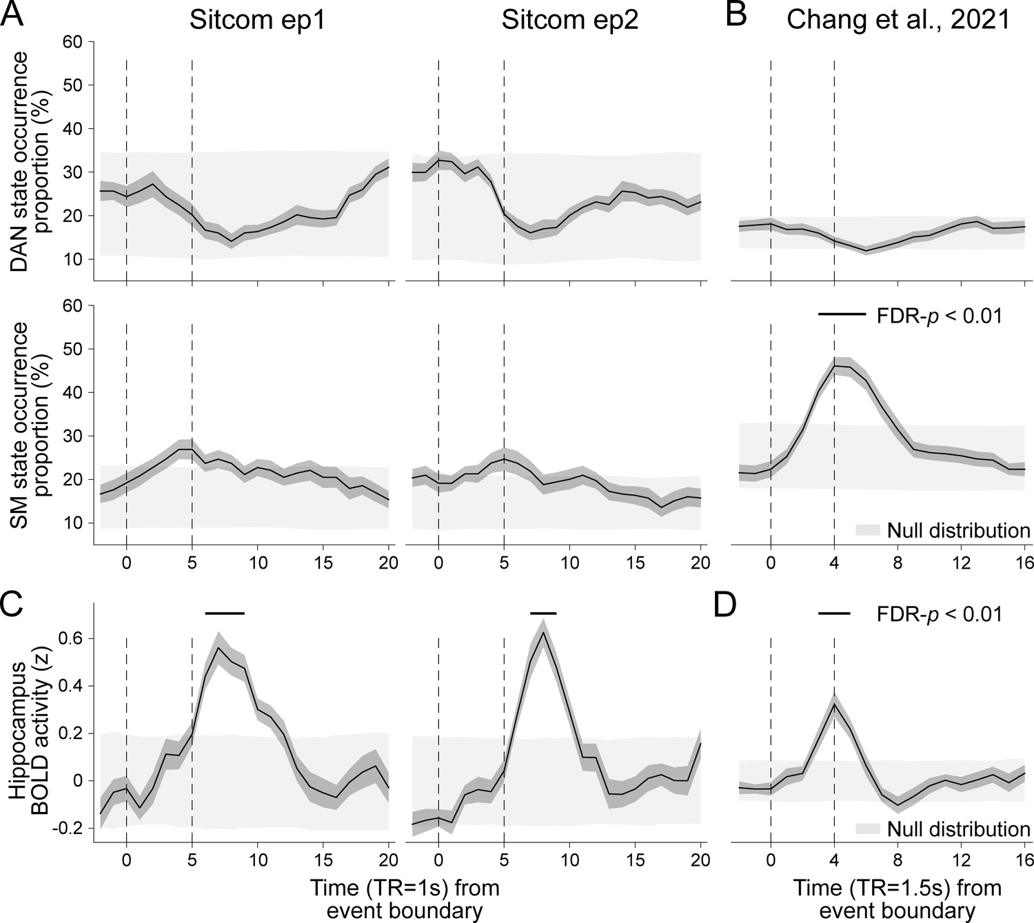
(A, B) Neural state occurrence after event boundaries. This figure complements Figure 4A and B, which only showed default mode network (DMN) and base state occurrence proportions. Consistent across (A) the sitcom episodes 1 and 2 runs in the SONG dataset and (B) the external dataset, Chang et al., 2021b, no change in the dorsal attention network (DAN) state occurrence was found after event boundaries. No change in the somatosensory motor (SM) state occurrence was found for the sitcom episodes 1 and 2. An increase in SM state occurrence after event boundaries is likely to be due to ~6 s of silent pauses in the audio in between the events. Given that the SM state occurred at intermittent rests in between the task blocks (Figure 5—figure supplement 1), the increase in the SM state after event boundaries may be due to a blank period rather than the narrative event change. (C, D) BOLD activity of the hippocampal ROI time course (z-normalized), time-aligned to narrative event boundaries of the (C) SONG dataset’s sitcom episodes and (D) audio story. The hippocampal ROI mask of the MNI template was adopted from Tian et al., 2020.
Figure 4—figure supplement 2
Transitions to the default mode network (DMN) state at narrative event boundaries.
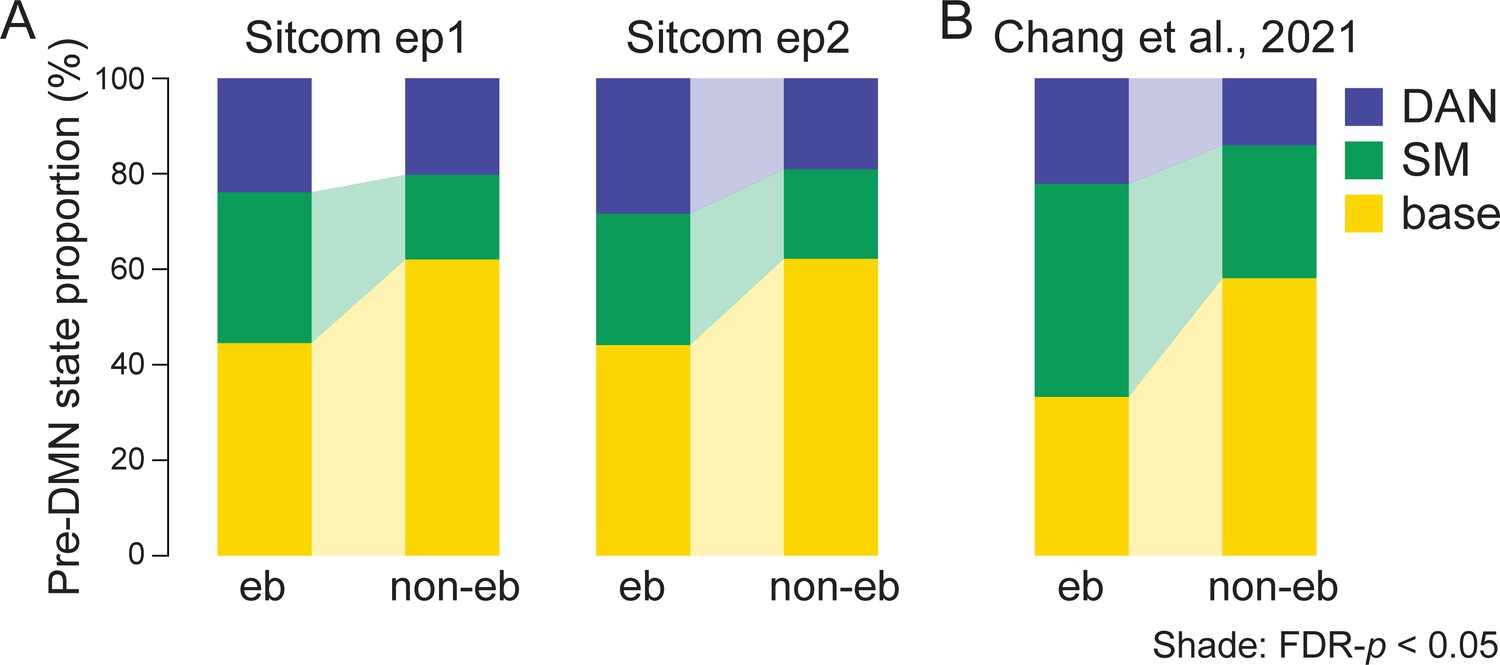
This figure complements Figure 4C, which visualizes the schematics of these results. (A) The proportion of the dorsal attention network (DAN), somatosensory motor (SM), and base states that occurred prior to the DMN state occurrence during the sitcom episodes 1 (left) and 2 (right). Transitions to the DMN state were categorized based on whether the DMN state occurred 5–15 TRs after the event boundaries (event boundary; eb) or not (non-event boundary; non-eb). Paired Wilcoxon signed-rank tests were conducted between the event boundary and non-event boundary conditions per neural state, and the significant difference is indicated with a colored shade (FDR-p<0.05). (B) Same as (A) but in Chang et al., 2021b dataset. Transitions to the DMN state 4–12 TRs after the event boundaries were compared to those that occurred at the rest of the moments. The proportions were averaged across participants for visualization.
Figure 5 with 1 supplement

Relationship between latent neural states and attentional engagement.
(A) Schematic illustration of the gradCPT and continuous narrative engagement rating. (Top) Participants were instructed to press a button at every second when a frequent-category image of a face or scene appeared (e.g., indoor scene), but to inhibit responding when an infrequent-category image appeared (e.g., outdoor scene). Stimuli gradually transitioned from one to the next. (Bottom) Participants rewatched the sitcom episodes and documentary after the fMRI scans. They were instructed to continuously adjust the scale bar to indicate their level of engagement as the audiovisual stimuli progressed. (B) Behavioral measures of attention in three fMRI conditions. Inverse RT variability was used as a measure of participants’ attention fluctuation during gradCPT. Continuous ratings of subjective engagement were used as measures of attention fluctuation during sitcom episodes and documentary watching. Both measures were z-normalized across time during the analysis. (C–G) Degrees of attentional engagement at moments of latent state occurrence. The attention measure at every time point was categorized into which latent state occurred at the corresponding moment and averaged per neural state. The bar graphs indicate the mean of these values across participants. Gray dots indicate individual data points (participants). The mean values were compared with the null distributions in which the latent state dynamics were circular-shifted (asterisks indicate FDR-p<0.01). (C, E, G) Results of the fMRI runs in the SONG dataset. (D, F) The hidden Markov model (HMM) trained on the SONG dataset was applied to decode the latent state dynamics of (D) the gradCPT data by Rosenberg et al., 2016 (N = 25), and (F) the Sherlock television watching data by Chen et al., 2017 (N = 16).
Figure 5—figure supplement 1
Latent state dynamics during cognitive task blocks, decoded from the hidden Markov model (HMM) trained on the SONG dataset.
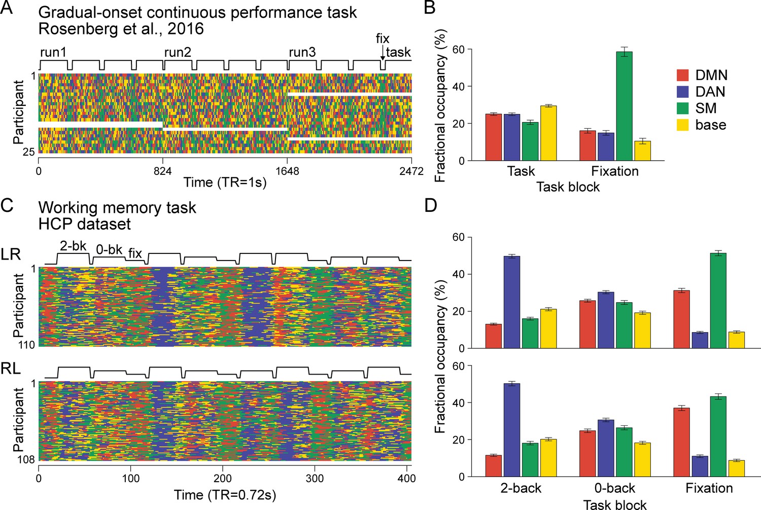
(A) Latent state dynamics of the gradCPT data collected by Rosenberg et al., 2016 (N = 25). The data consists of three runs, with each run consisting of four 3 min task blocks interleaved with 30 s of fixation. A boxcar plot indicates durations of the task and fixation blocks, shifted in time (5 TR; 5 s) to account for hemodynamic response delay. White areas indicate missing fMRI runs. (B) Fractional occupancies of the four states were calculated during task and fixation blocks separately and averaged across participants. The bar graph indicates the mean of fractional occupancies calculated per participant. The default mode network (DMN), dorsal attention network (DAN), and base states occurred more frequently during task than fixation blocks (paired t-tests, t(24) > 6, FDR-p-values<0.001), whereas the SM state occurred more frequently during fixation blocks (t(24) = 12.565, FDR-p<0.001). We observed a significant main effect of neural states (repeated-measures ANOVA: F(3,72) = 85.479, p<0.001) and an interaction between neural states and block types (F(3,72) = 119.392, p<0.001). The error bars indicate SEM. (C) Latent state dynamics of the Human Connectome Project (HCP) working memory (WM) task runs in left-to-right (LR; N = 110) and right-to-left (RL; N = 108) phase encoding sessions. Each session consists of a single run, with four 2-back WM (25 s), four 0-back WM (25 s), and three fixation blocks (15 s) interleaved, which are indicated in the boxcar plots shifted in time (6 TR; 4.32 s). (D) Fractional occupancies of the four states calculated at moments of 2-back WM, 0-back WM, and fixation blocks. In both sessions, DAN state occurrence decreased (paired t-tests for all block pairs, LR: t(109) > 13, RL: t(107) > 10, FDR-p-values<0.001), whereas the DMN and SM state occurrence increased (LR: t(109) > 3, RL: t(107) > 5, FDR-p-values<0.001), from 2-back to 0-back to fixation blocks as blocks required less cognitive control and memory load. The base state, on the other hand, occurred comparably during the 2-back and 0-back WM task blocks (LR: t(109) = 1.804, FDR-p=0.074, RL: t(107) = 1.486, FDR-p=0.140), whereas it occurred less at fixation blocks (LR: t(109) > 10, RL: t(107) > 9, FDR-p-values <0.001). The repeated-measures ANOVA showed the main effect of the neural states (LR: F(3,327) = 117.445, p<0.001; RL: F(3,321) = 126.702, p<0.001) and the interaction effect (LR: F(6,654) = 261.987, p<0.001; RL: F(6,642) = 149.786, p<0.001).
Author response image 1
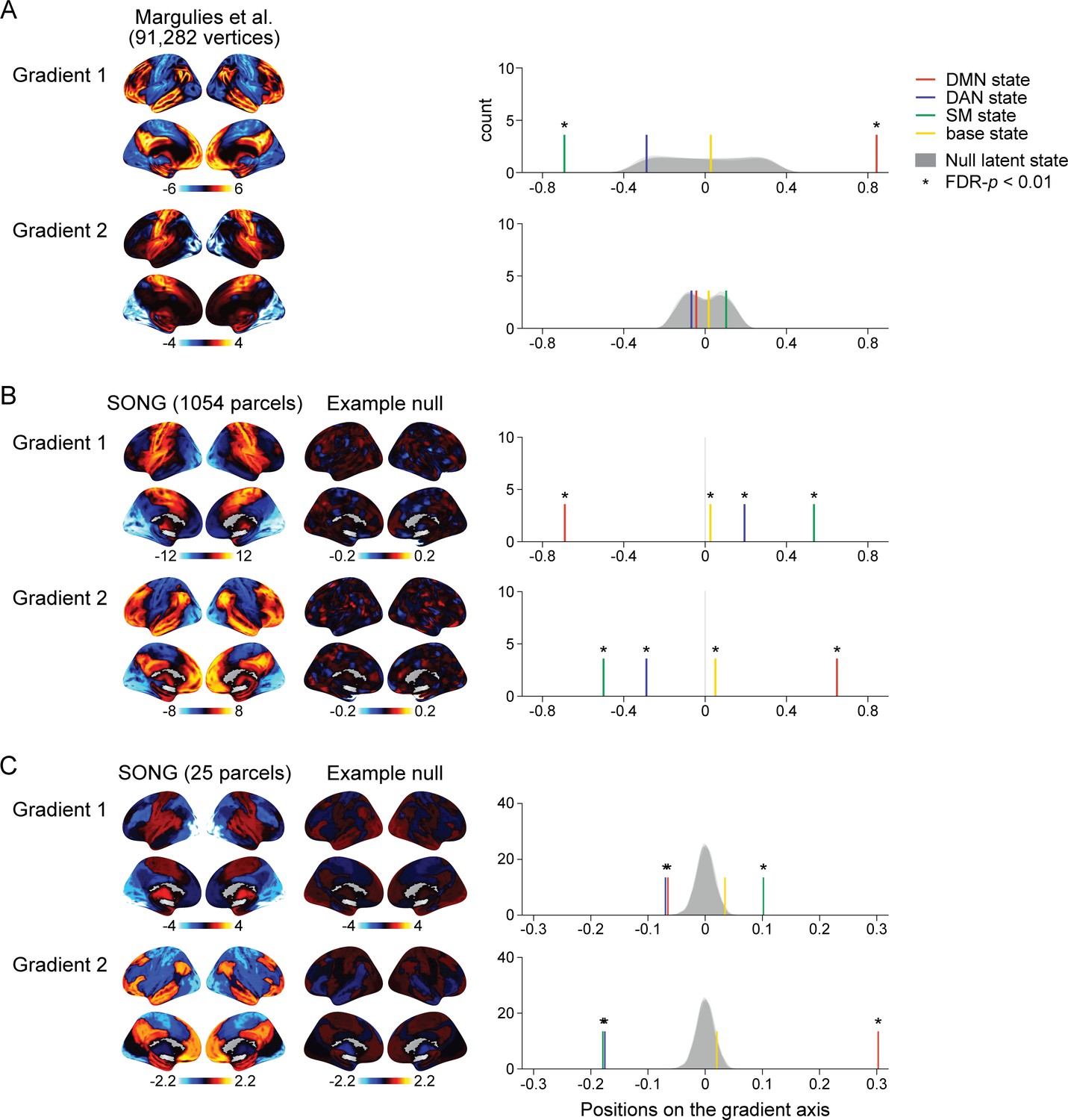
Test for the alignment between the latent states and the predefined and data-specific gradients.
(A) (Left) Visualization of the top 2 gradients of Margulies et al., 2016. (Right) Colored lines show the positions of the four latent states of the SONG dataset situated on the first and second gradient axes defined in Margulies et al., 2016. Four distributions (shown in overlap) indicate null hidden Markov model (HMM) states situated on the Margulies et al.'s (2016) gradient axes. Null states were generated by applying the HMM on the circular-shifted time series (1000 iterations; asterisks indicate FDR-p<0.01 compared to respective null distribution). (B) (Left) Visualization of the top 2 gradients of the SONG dataset, estimated based on the 1054 parcel time series. (Middle) Visualization of the example top 2 null gradients using 1054 parcels. Voxel time series were circular-shifted and then averaged per 1054 parcel to be used in null gradient estimation. (Right) Colored lines show the four states (HMM on the 25 parcel time series of the SONG dataset) situated on the top 2 gradient axes (gradients estimated from the 1054 parcel time series of the SONG dataset). A shared null model was generated by circular-shifting the voxel time series, which were averaged using 25 parcels for the latent state estimation or 1054 parcels for the gradient estimation. (C) (Left) Visualization of the top 2 gradients of the SONG dataset, estimated based on the 25 parcel time series also used in the HMM. (Middle) Visualization of the example top 2 null gradients using 25 parcels. Circular-shifted 25 parcel time series, used to estimate null HMM states, were also used to estimate functional connectivity gradients. (Right) Colored lines show the four states (HMM on the 25 parcel time series of the SONG dataset) situated on the top 2 gradient axes (gradients estimated from the 25 parcel time series of the SONG dataset). A shared null model was generated by circular-shifting 25 parcel time series.
Author response image 2
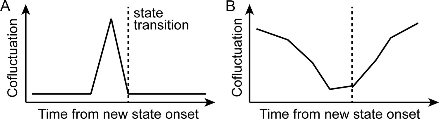
Schematics of the initial hypothesis and the observed result.
(A) Schematics of the initial hypothesis. We hypothesized that neural state transitions would be triggered by the transient increase in cofluctuation of selective pairs of brain regions. (B) Schematics of the observed results (Figure 2). We observed a global decrease in cofluctuation prior to state transitions.
Additional files
Download links
A two-part list of links to download the article, or parts of the article, in various formats.
Downloads (link to download the article as PDF)
Open citations (links to open the citations from this article in various online reference manager services)
Cite this article (links to download the citations from this article in formats compatible with various reference manager tools)
Large-scale neural dynamics in a shared low-dimensional state space reflect cognitive and attentional dynamics
eLife 12:e85487.
https://doi.org/10.7554/eLife.85487


