Robust membrane protein tweezers reveal the folding speed limit of helical membrane proteins
Figures
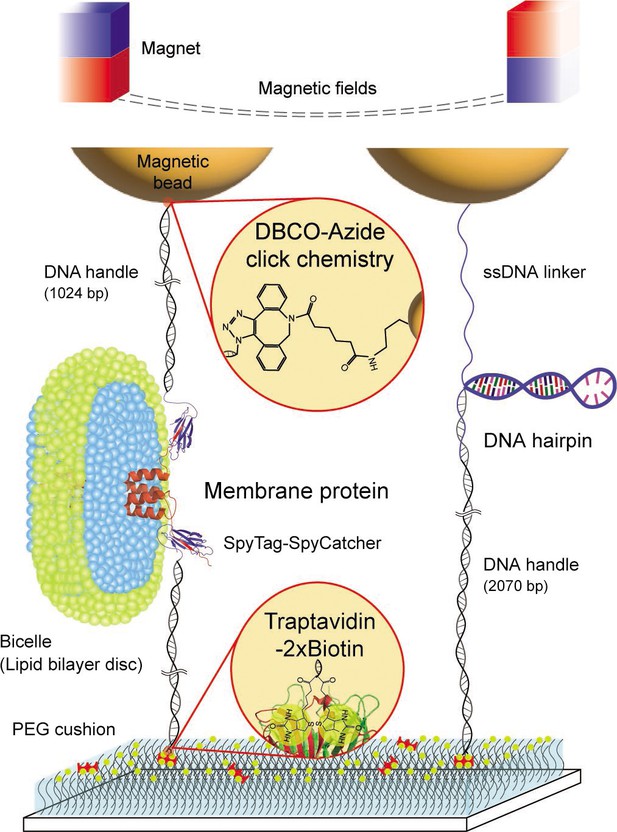
Schematic diagram of our robust single-molecule tweezers.
The tweezer approach was tested using two biomolecules of a membrane protein, scTMHC2, and a DNA hairpin, 17S6L. DNA handles are attached to the membrane protein via spontaneous isopeptide bond formation between SpyTag and SpyCatcher. A DNA handle is attached to the DNA hairpin via annealing and ligation. One end of the molecular constructs is tethered to magnetic beads via dibenzocyclooctyne (DBCO)-azide conjugation. The other end of the constructs is tethered to the sample chamber surface via traptavidin binding to dual biotins (2×biotin). The surface was passivated by molecular cushion of polyethylene glycol (PEG) polymers. The dashed lines on the top represent magnetic fields generated by a pair of permanent magnets. Lipids and detergents of the bicelle are denoted in blue and green, respectively.
-
Figure 1—source data 1
Original files of raw unedited gels and figures with uncropped gels.
- https://cdn.elifesciences.org/articles/85882/elife-85882-fig1-data1-v2.zip
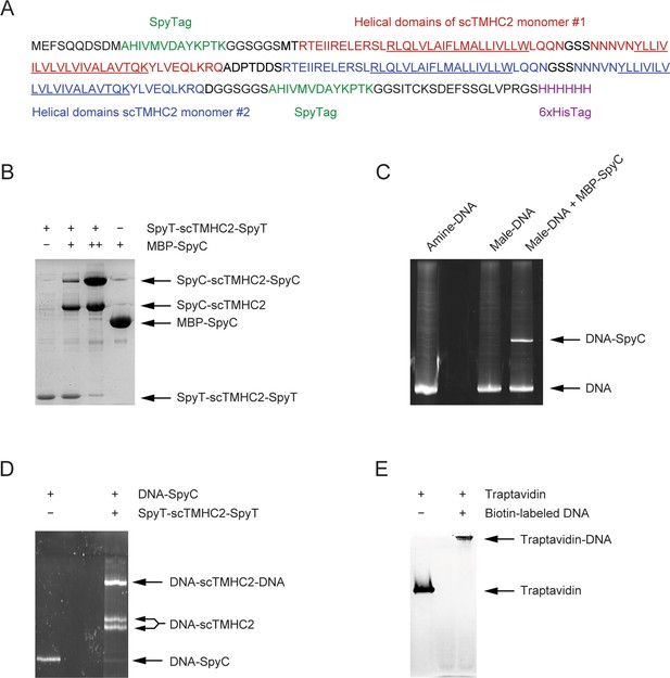
Preparation of molecular samples.
(A) Amino acid sequence of scTMHC2. The single-chained homodimer is composed of two same monomers with two helical domains. The underlined sequences correspond to transmembrane helical domains bounded by the RK and YW rings at the water-membrane interfaces. (B) Purification of scTMHC2 confirmed by 10% sodium dodecyl sulfate–polyacrylamide gel electrophoresis (SDS-PAGE). After protein purification, the binding test for SpyTag (SpyT) of scTMHC2 was performed by incubating with maltose binding protein (MBP)-fused SpyCatcher (MBP-SpyC). The doubly attached construct becomes dominant when a higher concentration of MBP-SpyC is added (denoted as ++). (C) DNA handle attachment to SpyCatcher confirmed by 6% SDS-PAGE. The amine-modified end of DNA is functionalized to maleimide (male) using an N-hydroxysuccinimide (NHS)-male crosslinker, followed by the attachment to the cysteine thiol of MBP-SpyC. The male-DNA indicates the DNA sample after the malemide functionalization and crosslinker removal. The yield of DNA-SpyC is ~30%. (D) DNA-SpyC attachment to scTMHC2 confirmed by 6% SDS-PAGE. The DNA handles conjugated to MBP-SpyC are attached to scTMHC2 via the binding between SpyT and SpyC. The two bands for the singly attached construct correspond to the N- and C-terminal attachments, respectively. ~50% of the doubly attached construct is the one with azide at one end and dual biotins (2×biotin) at the other end. Only this construct can be tethered to a magnetic bead and the chamber surface as shown in Figure 1. (E) Purification of traptavidin confirmed by 12% SDS-PAGE. After protein purification, the biotin-binding test was performed using 100 bp biotinylated DNA.
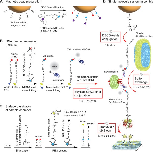
Procedure of single membrane protein tethering.
(A) Dibenzocyclooctyne (DBCO) modification on the surface of amine-coated magnetic beads. (B) Preparation of SpyCatcher-DNA handles. One end of the handles is labeled with amine, while the other end of the handles is labeled with azide or dual biotins (2×biotin). The amine end is modified by maleimide, followed by the attachment to the cystine of SpyCatcher which is fused to maltose binding protein (MBP). (C) Passivation of sample chamber surface. The surface is functionalized by amines via silanization, followed by polyethylene glycol (PEG) coating. (D) Assembly of single-molecule pulling system. The SpyCatcher-DNA handles are attached to a membrane protein solubilized in 0.05% n-Dodecyl-β-Maltoside (DDM) via SpyTag/SpyCatcher binding (first step). The hybrid molecular construct is bound to traptavidin at its 2×biotin-modified end. The remaining biotin-binding pockets of the traptativin are then attached to biotins on the surface (second step). The DBCO-modified bead is tethered to the other end of the molecular construct via DBCO-azide conjugation (third step). The final buffer exchange with bicelles allows for lipid bilayer environment for the membrane protein (fourth step).
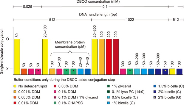
Single-molecule dibenzocyclooctyne (DBCO)-azide conjugation in detergent/lipid environments.
The DBCO concentration indicates the final concentration of DBCO-sulfo-N-hydroxysuccinimide (NHS) ester crosslinker in DBCO modification on bead surface. The other conditions, such as DNA handle length, membrane protein concentration, and detergent/lipid concentration, indicate those in DBCO-azide conjugation step of the single-molecule system assembly. Used buffers are a phosphate-buffered saline (100 mM sodium phosphate, 150 mM NaCl, and pH 7.3) and a Tris-buffered saline (50 mM Tris, 150 mM NaCl, and pH 7.5). The bicelle (C or G) consists of DMPC (or DMPG) lipid and CHAPSO detergent at a 2.5:1 molar ratio. The % indicates w/v %. The symbol O indicates successful conjugation between DBCO-modified beads and target membrane proteins. In this case, specifically tethered beads are found, and the force-extension curves of the molecular constructs are obtained (confirmed by three replicates). The symbol X indicates unsuccessful conjugation or entire nonspecific binding of beads to the surface. In this case, no data are obtained. See Figure 3—source data 1 for the full list. Abbreviations: DMPC, Dimyristoylphosphatidylcholine; DMPG, Dimyristoylphosphatidylglycerol; CHAPSO, 3-[(3-cholamidopropyl)dimethylammonio]-2-hydroxy-1-propanesulfonate.
-
Figure 3—source data 1
Full list of tested conditions for dibenzocyclooctyne (DBCO)-azide conjugation.
- https://cdn.elifesciences.org/articles/85882/elife-85882-fig3-data1-v2.zip
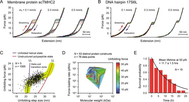
Robustness evaluation of our single-molecule tweezers.
(A and B) Representative force-extension curves of the membrane protein scTMHC2 (A) and the DNA hairpin 17S6L (B) at different magnet speeds (N=20 for each condition). The magnet speed is denoted as ms. (C) Scatter plot of unfolding forces and step sizes of the membrane protein (N=5 molecules, n=1000 data points, and ms = 0.5 mm/s). The blue and red lines represent the protein force-extension curves for the unfolded helical state (Uh) and the fully, unstructured polypeptide state (Up), respectively. (D) Survey of protein unfolding forces that were previously measured by single-molecule tweezers (N=53 distinct protein constructs, n=76 data points). See Figure 4—source data 1 for the full list. (E) Survival probability of our tethering system as a function of time. The mean lifetime of 11.7±1.5 (SE) hr at 50 pN was obtained by fitting the plot with exponential decay function (N=15).
-
Figure 4—source data 1
Survey of protein unfolding forces in optical and magnetic tweezers.
- https://cdn.elifesciences.org/articles/85882/elife-85882-fig4-data1-v2.zip

Force calibration and unfolding forces/sizes of scTMHC2.
(A) Force as a function of magnet height. The data was fitted by two-term exponential decay function (red). The error bars represent SD. (B and C) Count histograms of unfolding forces (B) and step sizes (C) at magnet speed of 0.5 mm/s (N=5 molecules, n=1000 data points). The Gaussian fitting yield the most probable unfolding force and step size (peak value ± SE).
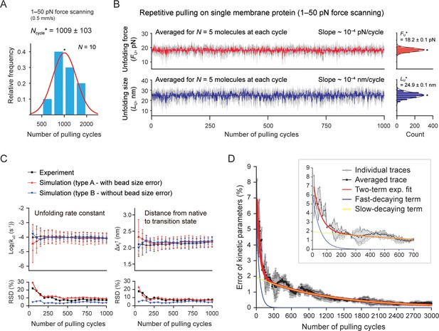
Stable single-molecule tweezers over a thousand pulling cycles.
(A) Applied number of pulling on single membrane protein until bead detachment (N=10 molecules). The peak value (Ncycle*) is 1009±103 (SE). The force-scanning range was 1–50 pN. The magnet speed was 0.5 mm/s. (B) Unfolding force and step size during progress of pulling cycles (analyzed for five molecules surviving more than the thousand cycles). The colored traces represent the averaged traces for five different molecules at each cycle. The SD at each cycle is denoted in gray. The slope of the traces was obtained as ~10–4 pN(nm)/cycle by linear fitting. Count histograms of the values are shown on the right (peak value ± SE). (C) Kinetic parameters during progress of pulling cycles (N=5 molecules). ku0 and Δxf† indicate the unfolding rate constant at zero force and the distance between the native and transition states, respectively. Relative SD (RSD) indicates the ratio of SD to mean. (D) Error of kinetic parameters during progress of pulling cycles. The gray traces indicate individual traces created from Monte Carlo (MC) simulations shown in Figure 5—figure supplement 5. The black trace is the trace averaged for the individual traces. The red curve represents the two-term exponential fitting. The blue and yellow curves represent the fast- and slow-decaying terms, respectively. The inset shows the initial hundreds of pulling cycles.
-
Figure 5—source data 1
Codes for the Monte Carlo simulations.
- https://cdn.elifesciences.org/articles/85882/elife-85882-fig5-data1-v2.zip
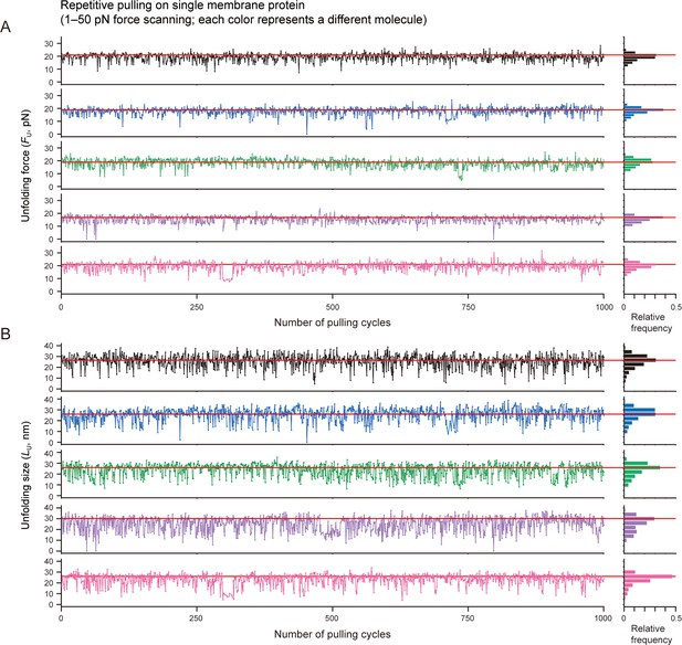
Unfolding force/size of individual proteins during progress of pulling cycles.
(A and B) Individual traces of the unfolding force plot (A) and unfolding size plot (B) shown in Figure 5B. Each color represents a different molecule. The same color code was used in panels A and B. Relative frequency histograms of the values are shown on the right (n=1000 data points for each). The horizontal lines indicate the bin center positions of the histogram peaks.

Unfolding/refolding forces during progress of pulling cycles for DNA hairpin.
The data were analyzed for five molecules surviving more than 1000 pulling cycles. The colored traces represent the averaged traces for five different molecules at each cycle. The SD at each cycle is denoted in gray. The slope of the traces was obtained as ~10–4 pN/cycle by linear fitting. Count histograms of the values are shown on the right (peak value ± SE).
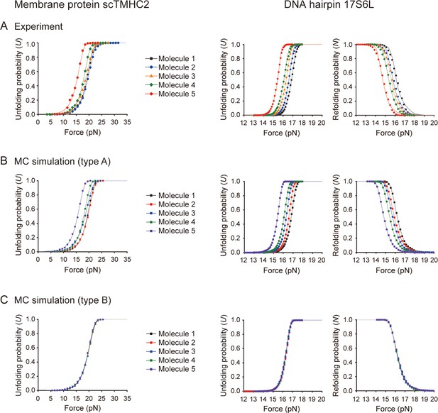
Unfolding/refolding probabilities as a function of force.
(A–C) Data obtained from experiments (A) and Monte Carlo (MC) simulations (B and C) (N=5 molecules; n=1000 or 1500 data points for membrane protein or DNA hairpin, respectively). In the type-A simulation, the unfolding/refolding force values were generated from all probability density functions (PDFs) obtained from the experiments, reflecting the bead size error. In the type-B simulation, the force values were generated from a median PDF with respect to the force at U=0.5, effectively removing the bead size error. The labels of molecules in the type-B simulation indicate the random sampling at different time points.

Comparison of two modes of kinetic analyses.
(A) Unfolding probabilities as a function of force for DNA hairpin that were obtained from all unfolding force data from all molecules (N=5 molecules, n=7500 data points; 1500 data points for each molecule). The plots from the experiment and simulation-type A (with bead size error) are deviated from that of the simulation-type B (without bead size error). The deviations yield wrong kinetic values, as shown in panel B. (B) Kinetic values obtained from the two modes of kinetic analyses. The analyzed kinetic parameters are the unfolding rate constant at zero force (ku0) and the distance between the native and transition states (Δxf†). The black squares indicate the average of kinetic values obtained from individual molecules (mode 1). The red triangles indicate the kinetic values obtained from the analysis for all data together, as shown in panel A (mode 2). In the simulation-type B, the obtained kinetic values are identical regardless of the modes of kinetic analyses. For the analysis mode 1, the results from experiment and simulation-type A match that of simulation-type B. However, the analysis mode 2, i.e., analyzing the large amount of data from different molecules at once, led to significant deviations from the true values. This could be attributed to the shape distortion of the unfolding probability profile that arises when analyzing all unfolding force values with errors due to the bead size variations. The errors represent SE.
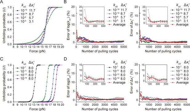
Error estimation of kinetic parameters.
(A and B) Kinetic errors for unfolding probability profiles with the same FU=0.5 and different slopes. For each set of kinetic values, the panels A and B show the unfolding probability as a function of force (A) and the kinetic error percentage during progress of pulling cycles (B), respectively. (C and D) Kinetic errors for unfolding probability profiles with the same slope and different FU=0.5. For each set of kinetic values, the panels C and D show the unfolding probability as a function of force (C) and the kinetic error percentage during progress of pulling cycles (D), respectively. All the data were created from the Monte Carlo (MC) simulation-type B since its results are consistent with those of experiment for the analysis mode 1, as shown in Figure 5—figure supplement 4. In panels B and D, the reference points of zero error are those for 10,000 times pulling. The error trace for each parameter set is the one averaged at each cycle for 10 simulations generated at different time points. The red curves are those averaged for the kinetic traces, which are shown as individual traces in Figure 5D.
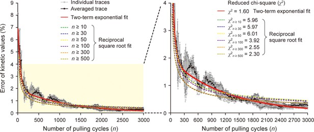
Comparison of two regression analysis models.
The plot of Figure 5D was analyzed by two regression models of two-term exponential function (y=A1∙exp[–n/τ1]+A2∙exp[–n/τ2]) or reciprocal square root function (y=A/ ). The red curve represents the two-term exponential fitting. The dashed curves represent the reciprocal square root fitting for different analyzed regions. The notation n≥N indicates that only the data points more than N pulling cycles were fitted by the model function. All the reciprocal square root fit functions were drawn for n≥30 for comparison. The right panel is the zoomed-in plot of yellow boxed region of the left panel. The reduced χ2 values are shown for a goodness-of-fit test (χ2=1 for the best fit).
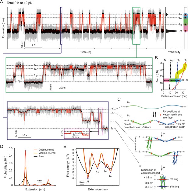
Structural transitions of scTMHC2 for 9 hr at 12 pN.
(A) Time-resolved extension trace of scTMHC2. The gray and black traces are the raw trace and median-filtered trace with 4.5 Hz window, respectively. The red lines indicate the state positions determined by the hidden Markov modeling (HMM) analysis. The probability density of the extension is shown on the right. The peak positions (black dots) with error bars (SD) are compared with the polymer model-estimated positions for each state (red lines). The color code for each transition is same as in panel B. The below insets are the zoomed-in plots for corresponding time regions. (B) Protein force-extension curves estimated by the worm-like chain (WLC) and Kessler-Rabin (KR) models. The curves for each state are denoted as the colored lines with dots. The transitions between the states at 12 pN are shown as arrows with colored backgrounds (pink, green, and blue). The yellow thick curve represents the helix-coil transition zone in the stretching experiments shown in Figure 4C. (C) Predicted structural states of scTMHC2 for the four extension positions at 12 pN. The RK and YW ring were designed to be positioned at the water-membrane interfaces. The gray arrows indicate the direction of applied force to the protein. The black arrows represent the allowed transitions between the states. (D) Probability density of protein extension obtained using the deconvolution method. (E) Folding energy landscape obtained from the deconvoluted probability density and Boltzmann relation.
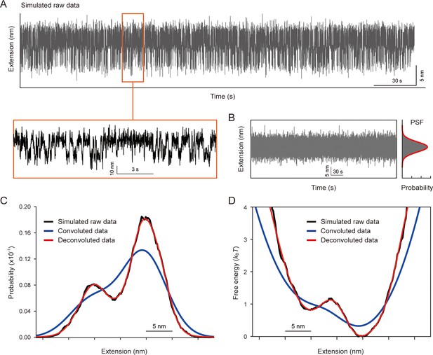
Evaluation of our deconvolution method using simulated traces.
(A) Two-state extension trace with dwell time constants of 0.33 s for the folded state and 0.14 s for the unfolded state. The two states have a 10 nm extension gap and a SD of 3 nm for the noise strength. The below inset shows the zoomed-in plot for the corresponding region. (B) Extension trace for point spread function (PSF). The probability density of extensions was fitted by the Gaussian function (right), which was used for the deconvolution process. (C) Raw, convoluted, and deconvoluted probability densities of extensions. The black, blue, and red curves indicate the probability densities of extensions obtained from the simulated raw data, after convolution with the PSF, and after deconvolution using our deconvolution method, respectively. (D) Free energy landscapes obtained from the probability densities using the Boltzmann relation. Our deconvolution method successfully restored the original probability density and energy landscape that were blurred by the PSF.
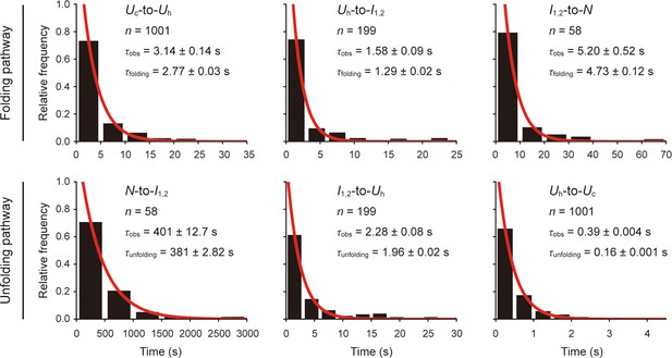
Folding and unfolding times of scTMHC2 at 12 pN.
The dwell times of one state until transitioning to another state were obtained from the hidden Markov modeling (HMM) analysis for the 9 hr-long trace at 12 pN. The observed (un)folding time (τobs) for each transition was obtained as the time constant for each dwell time distribution. The molecular (un)folding time (τ(un)folding) was obtained by correcting τobs for the limited temporal resolution and tethered bead-handle effect. The errors represent SE.

Average penetration angle and depth of helices of the Uh state at 12 pN.
See Methods for more details for this estimation. The protein extension of the Uh state is the measured step size from the N state at 12 pN. The two helices of each monomer are colored green and blue. The Dhelix and <Dhelix,w> represent the contour length of helices and the average contour length of the soluble parts of helices on the pulling side, respectively. The <θp> and <dp> represent the average penetration angle and depth of helices into the membrane, respectively. The arrows denote the direction of force application. The bicelle core represents the lipid tail part of bicelle. The errors represent SE.
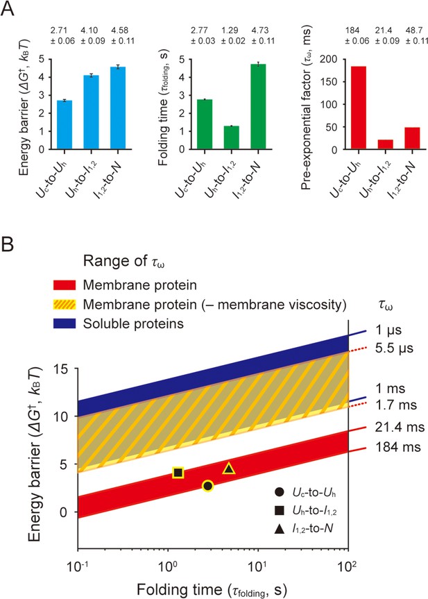
Estimation of pre-exponential factors for scTMHC2 folding transitions.
(A) Energy barriers, folding times, and pre-exponential factors of the transitions. The energy barrier heights (ΔG†) were obtained by the deconvolution method. The folding times (τfolding) were obtained by the hidden Markov modeling (HMM) analysis and instrumental error correction. The two measured parameters yield the pre-exponential factors (τω) of the Kramers equation for the folding transitions. The error bars represent SE. (B) ΔG†–τfolding plane showing the regions for designated τω ranges. The black data points indicate the measured values of ΔG† and τfolding. The red-shaded area, yellow-shaded area with slash lines, and blue-shaded area correspond to the regions for the estimated τω range, the τω range in the absence of lipid membrane viscosity (denoted as ‘– membrane viscosity’), and the τω range observed for soluble proteins, respectively.
-
Figure 7—source data 1
Survey of measured viscosity for DMPC lipid membranes.
- https://cdn.elifesciences.org/articles/85882/elife-85882-fig7-data1-v2.zip


