Continuous odor profile monitoring to study olfactory navigation in small animals
- Princeton Neuroscience Institute, Princeton University, United States
- Department of Physics, New York University, United States
- Center for Neural Science, New York University, United States
- Department of Physics, Princeton University, United States
Figures
Figure 1 with 6 supplements
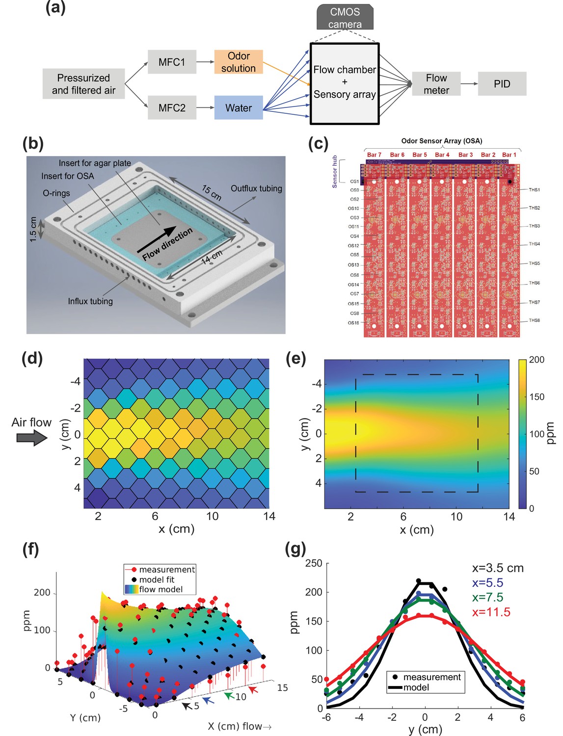
Odor flow chamber with controlled and measured odor concentration.
(a) Schematic of airflow paths. Airflow paths for odor solution and water are controlled separately by mass flow controllers (MFCs) and spatially arranged into the odor chamber. The outflux from the chamber connects to a flow meter and photo-ionization detector (PID). (b) Flow chamber design. (c) Odor sensory array (OSA). Seven odor sensor (OS) bars are connected to a sensor hub. Each bar has 16 OS and 8 temperature/humidity sensors (THS). Measured odor concentrations from the OSA of a spatially patterned butanone odor concentration shown in (d) for each sensor, (e) interpolated across the arena with square dashed line indicating the area where agar and animals are placed. (f) A two-parameter analytic flow model fit to measurement. (g) Cross-sections from (f) at four different x-axis positions (shown as colored arrows). Sensor readouts are overlaid points on the smooth curves from a 1D diffusion model.
Figure 1—figure supplement 1
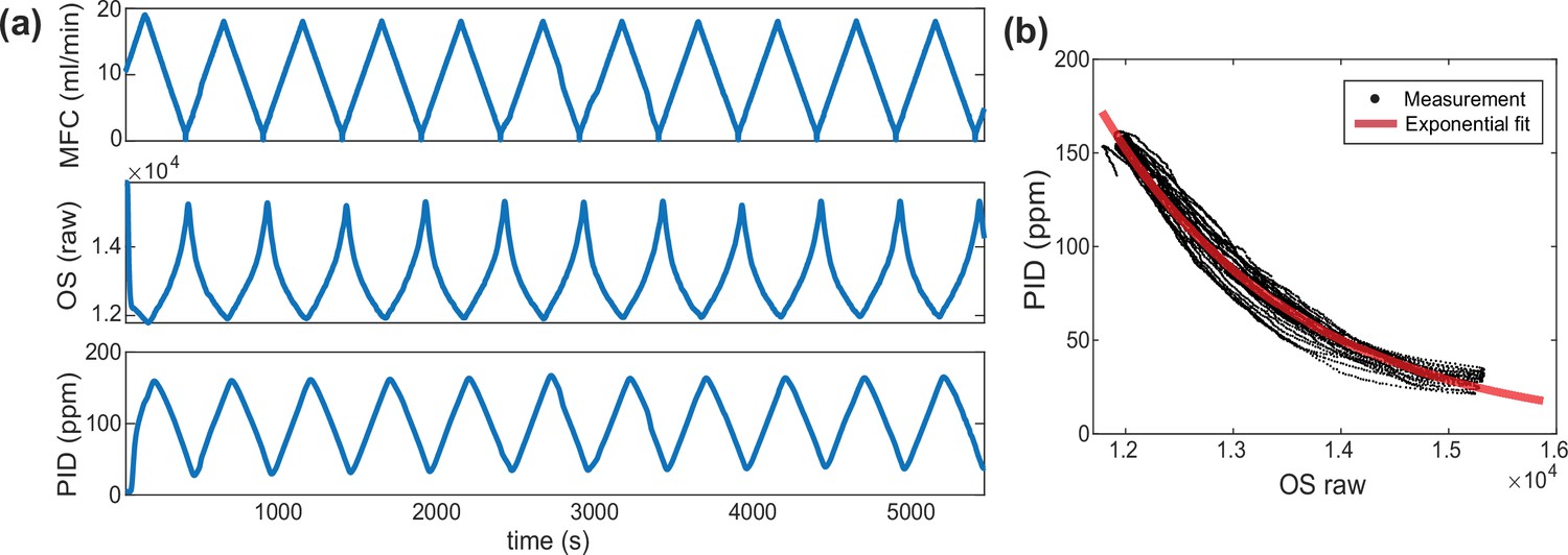
Long-term agreement between photo-ionization detector (PID) and metal-oxide sensors (odor sensor, OS).
(a, top) Butanone odor flow rate driven by the mass flow controller (MFC), (a, middle) raw reading of an OS located in the chamber, (a, bottom) odor concentration readout from the PID located at the outlet of the chamber. Note that the measurement is stable across the 90 min recording. (b) We correct for the time lag between sensors and plot the mapping between PID measurements and OS readings.
Figure 1—figure supplement 2

Temporal response of odor sensor (OS) to a step in odor concentration.
(a, top) Butanone odor flow rate driven by the mass flow controller (MFC), (a, middle) raw reading of an OS located in the chamber, (a, bottom) odor concentration readout from the photo-ionization detector (PID) located at the outlet of the chamber. (b) Row OS temporal response to steps is reliable and qualitatively similar to the PID. Step responses are extracted from (a) at time points indicated by gray dashed lines. The OS and PID traces have been scaled and note the OS trace has been inverted. Since the PID is located spatially downstream, we expect the PID to respond delayed in time. (c) We correct for the time lag between sensors and plot the mapping between PID measurements and OS readings from the second half (300 s) of each stepping phase.
Figure 1—figure supplement 3
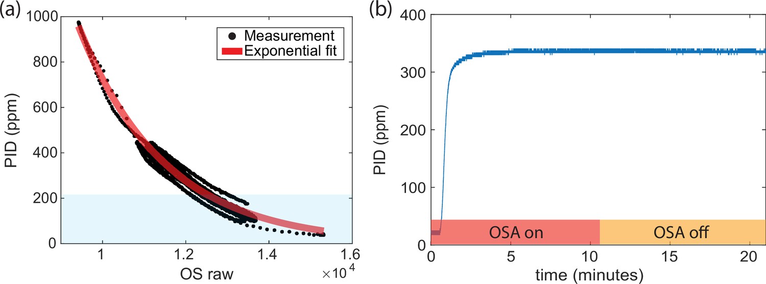
Additional odor sensor controls.
(a) Odors used in this work (shaded region) fall well within the dynamic range of the odor sensors. (b) Turning on the odor sensors has no detectable impact on the downstream odor concentration as measured by the photo-ionization detector (PID).
Figure 1—figure supplement 4
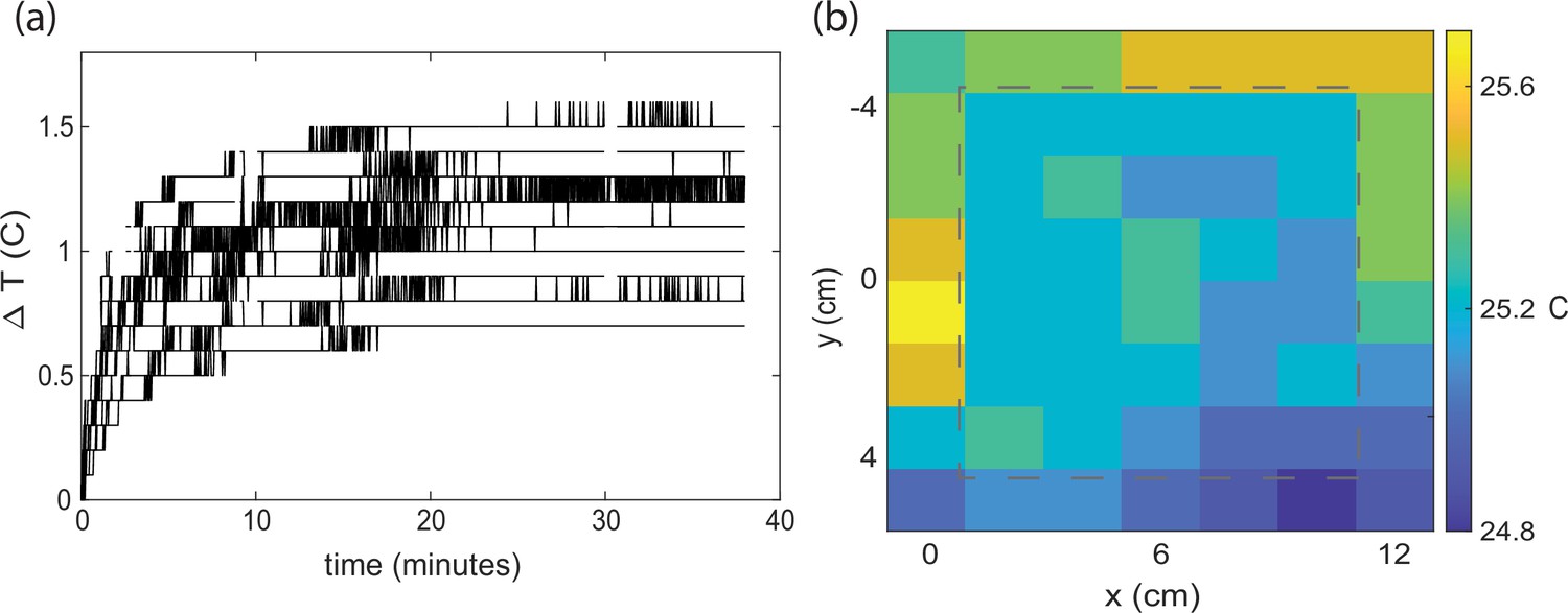
Characterization of temperature landscape.
(a) Temperature change is measured from the thermo-hydro sensors on the odor sensor bars in the arena upon activating the odor sensors. (b) Spatial temperature distribution across the array at time 20 min in (a). The gray dash line shows where the agar plate would be positioned during animal experiments. Heating is most prominent in the upper right corner near the odor sensor hub, which has less thermal contact with the optics table. We expect the heating shown here to represent an upper bound for agar experiments with animals, because here all 112 odor sensors were active and generating heat, while with agar experiments only 32 odor sensors would be active. Consistent with this, during separate experiments with agar, the temperature measured via a thermocouple at the four corners of the agar surface showed a difference in temperature within 0.4°C at four corners that are 10 cm apart.
Figure 1—figure supplement 5
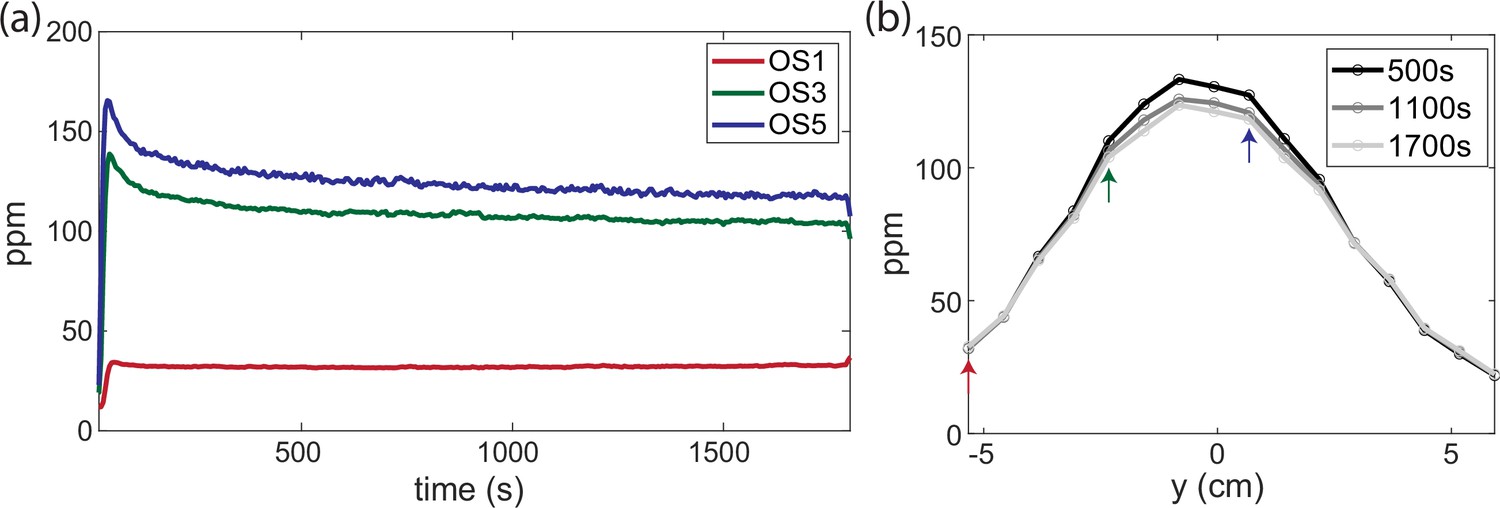
Odor profile is stable through time.
(a) Butanone concentration measured from three example odor sensors on an odor sensor bar (bar 5) across 30 min from the initial odor flow that forms a cone shape. (b) Cross-section along an odor sensor bar at three different time points that are 10 min apart. The three-colored arrows indicate odor sensors shown in (a).
Figure 1—figure supplement 6
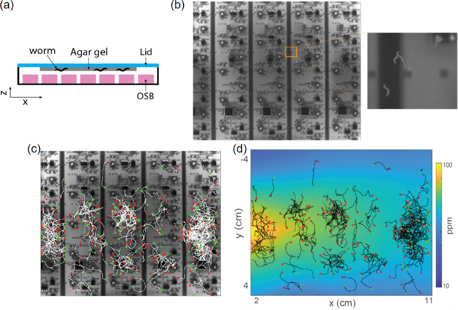
Behavioral measurement is challenging in the presence of the full sensor array.
(a) The schematic for recording with the full sensor array, agar gel, and worms. This is the same configuration as in Figure 6 but with simultaneous animal experiments. (b) Example frame from recording of worms on an agar gel on the lid with sensors underneath. Zoomed in region shows that worms only show greater contrast in the images in certain regions. (c) Example worm trajectories measured under the configuration in (a). Green dots are each animal’s initial positions and red dots are the endpoints. (d) Same as (c) but overlaid on top of the butanone odor landscape measured from the full sensor array.
Figure 2 with 1 supplement

Flexible control of a steady-state odor landscape.
(a) Configuration for a narrow cone with butanone. Colorbar shows interpolated odor concentration in ppm as measured by the odor sensor array. (b) An inverse cone landscape that has higher concentration of butanone on both sides and lower in the middle. Stationary cone-shape odor landscape of three different odorants: (c) benzaldehyde, (d) ethanol, and (e) ethyl butyrate.
-
Figure 2—source data 1
Physical properties of odorants.
Table odor_physics.xlsx in https://doi.org/10.6084/m9.figshare.21737303.
- https://cdn.elifesciences.org/articles/85910/elife-85910-fig2-data1-v2.xlsx
Figure 2—figure supplement 1
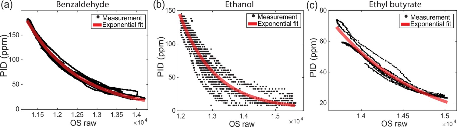
Odor sensor (OS) calibration for different odorants.
Mapping between photo-ionization detector (PID) measurements and OS readings for (a) benzaldehyde, (b) ethanol, and (c) ethyl butyrate. The concentration curves are produced with the same calibration protocol shown in Figure 1—figure supplement 1.
Figure 3 with 2 supplements

The presence of agar in the droplet assay alters the time evolution of butanone odor landscape.
(a) Schematic showing configuration of an odor droplet in an arena with or without agar. Red dot indicates the position of butanone droplet (2 µL of 10% vol/vol butanone in water) on the lid (blue) or agar (gray). Odor sensor bars are shown in purple. (b) Spatial concentration measured by odor sensor array is reported immediately after butanone droplet is introduced into the arena. (c) Spatial concentration after 3 min.
Figure 3—figure supplement 1
Concentration measurements with an odor droplet and experimental perturbation.
(a) The initial concentration readout from a droplet of butanone on the lid near the middle of the arena. (b) Same condition as (a), but 20 min after the recording (left) and after shortly opening and closing the lid back (right) to mimic perturbation during worm experiments. (c) When there is agar in the chamber, the odor concentration is better maintained in the chamber. Location of the odor droplet is shown with a red dot. (d) After 20 min of recording (left) and after shortly opening and closing the lid back (right) to mimic experimental perturbation.
Figure 3—video 1
Time evolution of odor landscape from a butanone droplet placed on agar (right) and without agar (left).
The experimental conditions are the same as the first two rows of Figure 3. Blank sensor positions indicate sensors replaced by agar. The video updates every 2 s and measures butanone concentration from a droplet in the first 3 min. Video available online at https://vimeo.com/830670531.
Figure 4 with 1 supplement
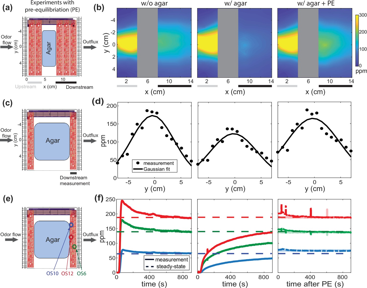
Under flow, agar interacts with butanone odor to disrupt the downstream spatial odor profile, but a pre-equilibration (PE) protocol can coax the system into quasi-equilibrium and restore a temporally stable odor profile.
(a) Two odor sensor bars are replaced with agar to observe the effect of introducing agar on the downstream spatial odor profile. (b) Measured butanone odor profile is shown upstream and downstream of the removed odor sensor bars in the absence (left) and presence of agar (middle). Transiently delivering a specific higher odor concentration ahead of time via a PE protocol restores the downstream odor profile even in the presence of agar. (c) Additional odor sensor bars are removed and replaced with a larger agar, as is typical for animal experiments. (d) Measurements from the downstream sensor bar under the same three conditions in (b). The dots are sensor measurements and the smooth curve is a Gaussian fit. (e) The same experimental setup in (a), here focusing on time traces of only three downstream odor sensors (colored circles for selected OS). (f) Concentration time series of three sensors color-coded in (e). Traces for three conditions are shown: time aligned to initial flow without agar (left), time aligned to initial flow with agar (middle), and traces after PE (right, with transparent line showing measurements another 20 min after the protocol). The dash lines indicate the target steady-state concentration for each sensor.
Figure 4—figure supplement 1
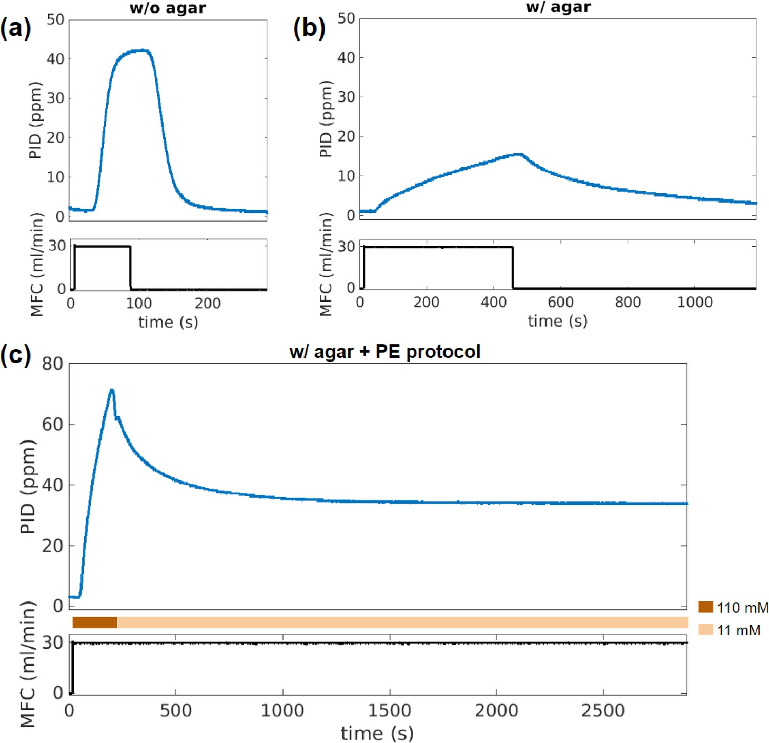
Time series of concentration change that capture effects of agar gel and the pre-equilibration (PE) protocol.
(a) Concentration readout from the downstream photo-ionization detector (PID) (top) in response to the impulse of airflow rate through the odor bottle controlled by mass flow controller (MFC) (bottom), with no agar in the flow chamber. The background clean airflow is constant ∼400 mL/min throughout the recording. (b) Same as (a) but with agar plate in the flow chamber. Note that the response timescales to the same impulse are significantly different. (c) The time trace recorded from the PE protocol with agar plates. Odor reservoir with high butanone concentration (110 mM) is applied in the beginning, swapped back to the target concentration (11 mM) at ∼200 s, the odor concentration readout relaxes and stabilizes after ∼900 s, which enters steady state for a duration longer than animal experiments.
Figure 5
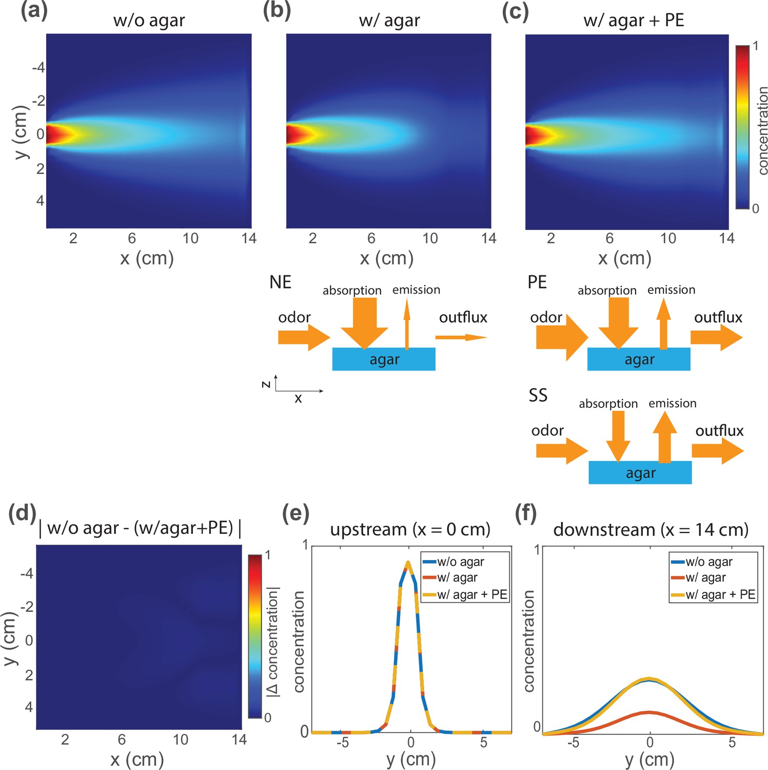
Simulations from a reaction-convection-diffusion model of odor-agar interaction show that at quasi-equilibrium the airborne odor concentration is the same with or without agar.
(a) Simulation results of steady-state odor concentration in air without agar and with flow configured as in Figure 1. (b) The same simulation condition in (a) but now shortly after agar is introduced and before quasi-equilibrium is reached. A schematic of odor-agar interaction model is shown below. When agar is introduced, it absorbs the odor in air and decreases concentration measured downstream, producing a non-equilibrium (NE) concentration profile. (c) Odor concentration profile in air, with agar present, but after the pre-equilibration (PE) protocol brings this system to quasi-equilibrum. The PE protocol is shown in the schematic below, followed with steady state (SS) with the stable odor concentration profile shown above. (d) The absolute difference of concentration profile without agar (a) and with agar after PE (c) is shown. (e) Upstream and (f) downstream odor concentrations along the agar boundary are shown for all three conditions.
Figure 6 with 1 supplement
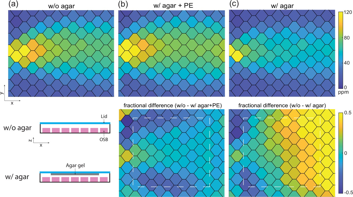
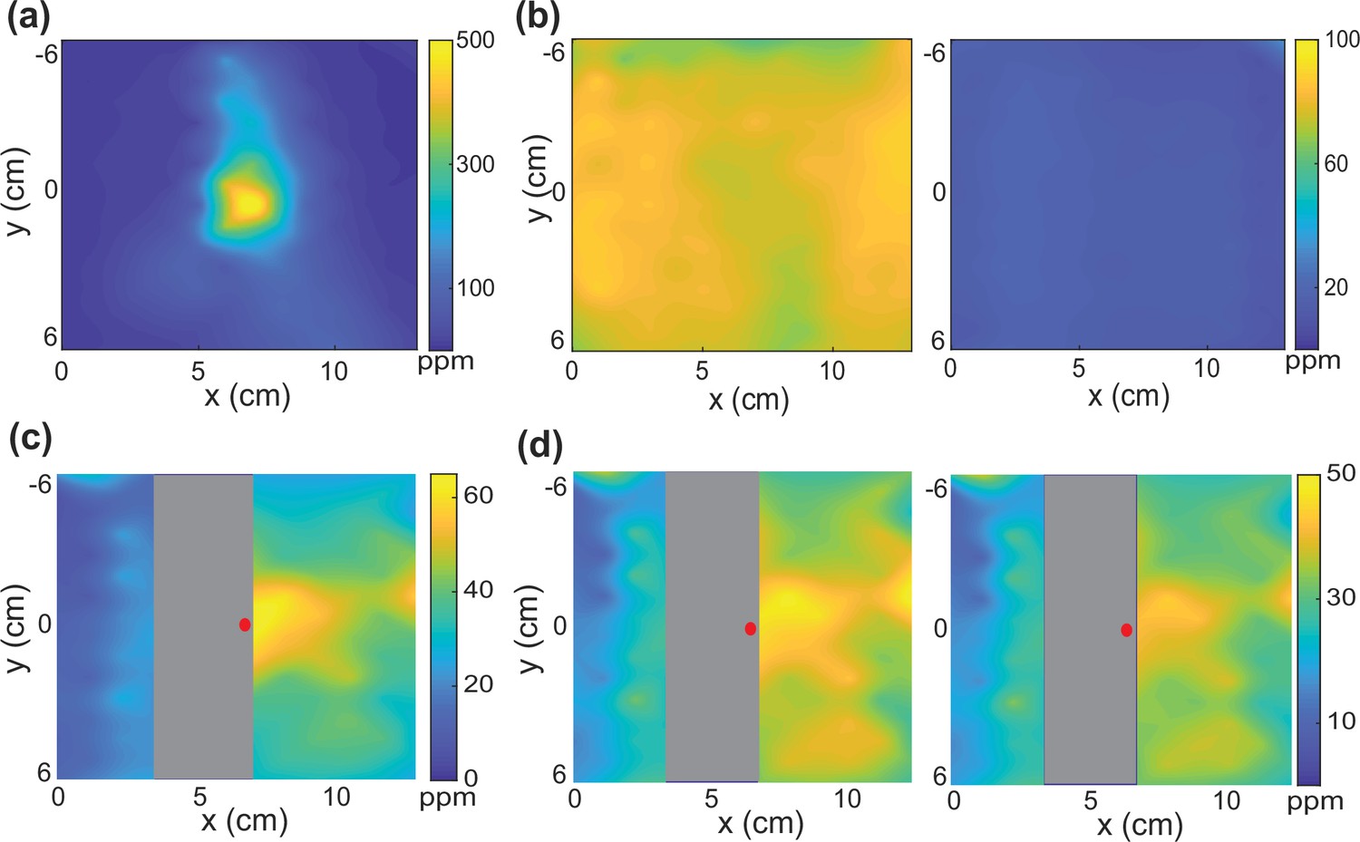
Direct measurement of odor concentration across agar confirms quasi-equilibrium odor profile.
(a) Stationary butanone odor-cone profile without agar. Schematic for configuration with or without agar in this direct measurement shown below. (b) Same as (a) but with agar on the lid after the pre-equilibration (PE) protocol. Fractional difference between odor profile with and without agar is shown below and white dash line indicates the region with agar gel. (c) Same as (b) but without the PE protocol, 15 min into the recording. Fractional difference and agar gel region is shown below.
Figure 6—figure supplement 1
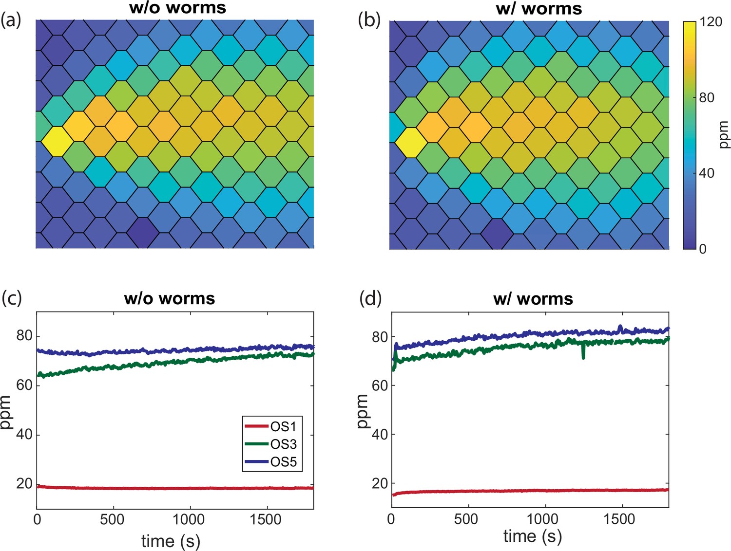
Quasi-equilibrium odor profile with agar is stable during animal experiments.
(a) Stationary butanone odor-cone profile with agar after the pre-equilibration (PE) protocol. (b) Same as (a) but during simultaneous worm behavioral experiments. (c) Time traces of concentration measured from (a), showing three example odor sensors on an odor sensor bar (bar 6) across 30 min. (d) Same as (c) but from measurements with worm experiments in (b).
Figure 7 with 2 supplements
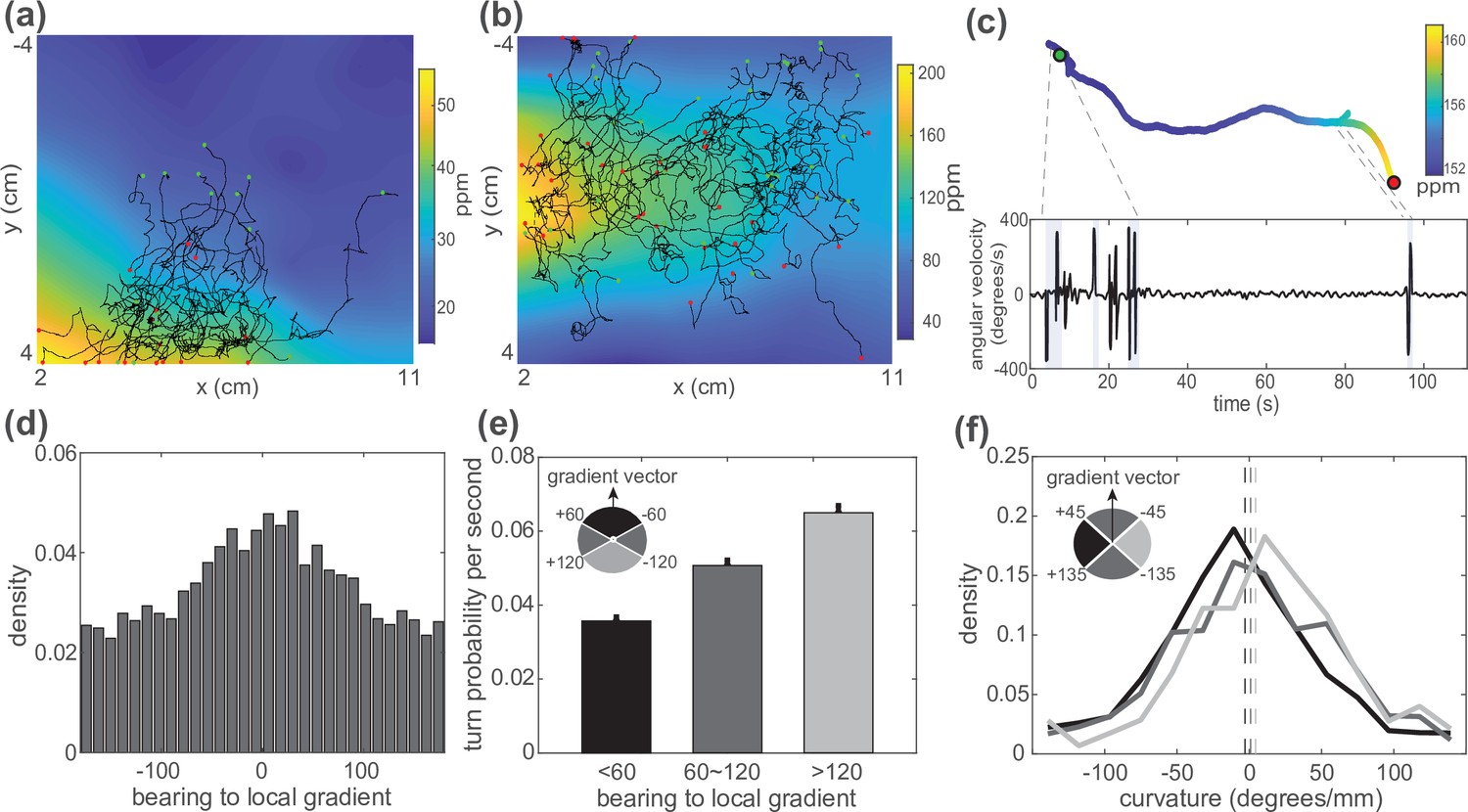
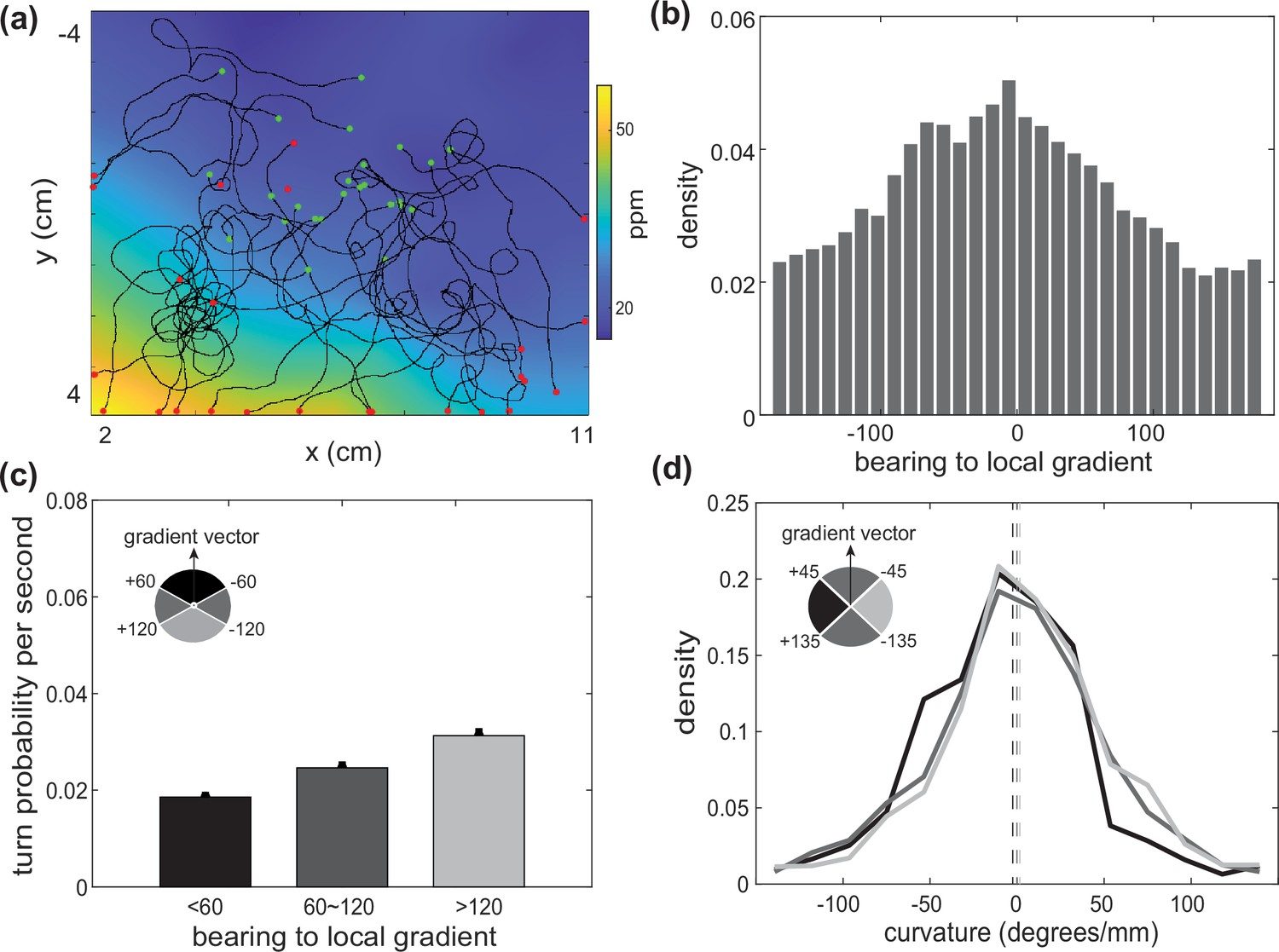
C. elegans use both biased random walk and weathervaning to navigate in a butanone odor landscape.
Animals on agar were exposed to butanone in the flow chamber. (a, b) Measured animal trajectories are shown overlaid on airborne butanone concentration for different odor landscapes. Green dots are each animal’s initial positions and red dots are the endpoints. (c) An animal’s trajectory is shown colored by the butanone concentration it experiences at each position (top). Its turning behavior is quantified and plotted over time. Turning bouts are highlighted in gray. (d) Distribution of the animal’s bearing with respect to the local airborne odor gradient is shown. Peak around zero is consistent with chemotaxis. (e) Probability of observing a sharp turn per time is shown as a function of the absolute value of the bearing relative to the local gradient. Modulation of turning is a signature of biased random walk. Error bars show error for counting statistics. Data analyzed from six experiments, ∼100 worms per experiment, resulting in over 90 animal-hours of observation. (f) Probability density of the curvature of the animal’s trajectory is shown conditioned on bearing with respect to the local gradient. Weathervaning strategy is evident by a skew in the distribution of trajectory curvature when the animal travels more perpendicular to the gradient. Bearing to local gradient defined by gray-scale quadrants. Three distributions are significantly different from each other according to two-sample Kolmogorov-Smirnov test (). Means are shown as vertical dashed lines.
Figure 7—figure supplement 1
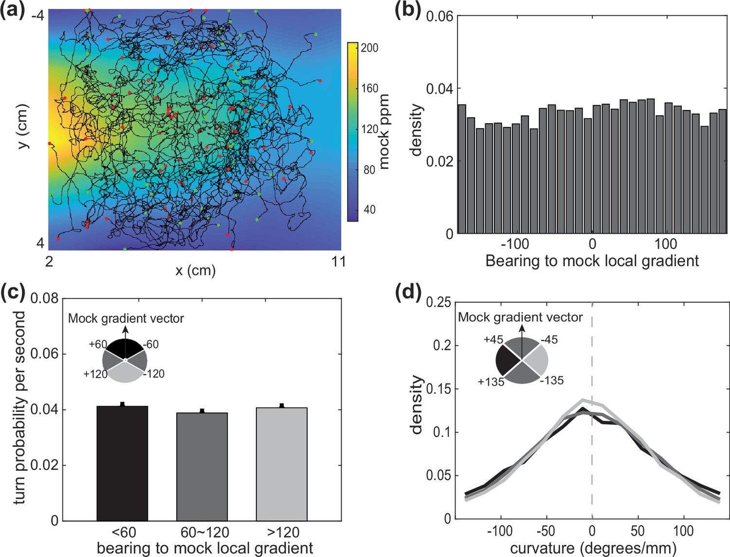
Control measurements with airflow but no odor.
(a) Behavioral trajectories overlaid on the odor landscape that would have been expected had odor been present (mock odor landscape). No odor is presented, only moisturized airflow. (b) Distribution of bearing to the mock gradients under clean airflow. (c) Turn probability at different bearing conditions to the mock gradient. (d) Curvature conditioned on different bearing measurements. Data analyzed from two experiments, ∼200 worms per experiment, resulting in over 159.4 animal-hours of observation.
Figure 7—figure supplement 2
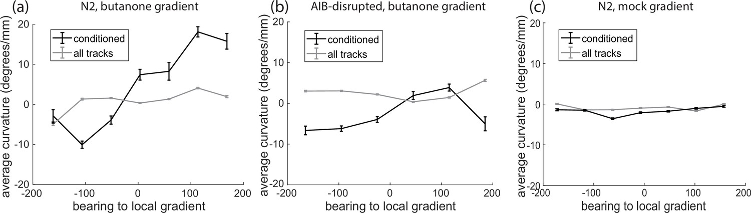
Characterizing weathervaning with average curvature.
(a) Average curvature as a function of bearing to local gradients. This is calculated for all tracks or for only those time points when the gradient is larger than one standard deviation above the mean calculated from all tracks (conditioned). Error bars show standard error of the mean. (b) Same calculation as (a) for worms with down-regulated AIB neuron. (c) Same calculation as (a) for environment with airflow but no odor.
Figure 8
Butanone chemotaxis in worms with down-regulated AIB neuron.
(a) Example behavioral trajectories from worms with down-regulated AIB neuron in the same butanone landscape. Green dots are each animal’s initial positions and red dots are the endpoints. (b) Distribution of bearing to local gradients. (c) Turning probability at different bearing conditions. (d) Curvature conditioned on different bearing measurements. Data analyzed from three experiments, ∼100 worms per experiment, resulting in over 51 animal-hours of observation.
Figure 9

Chemotaxis performance as a function of gradient steepness.
(a) Schematic of a worm tracked in the odor landscape. The crawling velocity vector , local concentration gradient , bearing angle , and drift velocity are shown. (b) Tuning curve shows the drift velocity as a function of the odor concentration gradient. Gray dash line indicates an unbiased performance with zero drift velocity, gray dots are the discrete measurements, and the black line shows the average value within bins. Error bar shows lower and upper quartiles of the measurements. Other than the left-most bin with the lowest gradient, all other bins show significant difference from zero drift velocity using t-test (p<0.001, ***). Both two-sample t-test and Kolmogorov-Smirnov test (given the non-Gaussian distribution) show significant differences between bins and the first bin with the lowest concentration gradient (p<0.001).
Figure 10
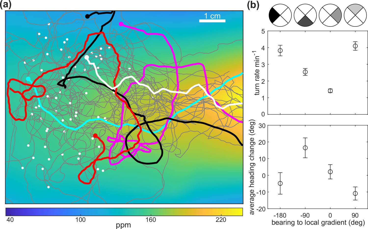
D.melanogaster larvae chemotaxis in the odor flow chamber.
(a) Trajectories overlaid on the measured butanone odor concentration landscape. Example tracks are highlighted and the initial points are indicated with white dots. (b) Top: turn rate versus the bearing, which is the instantaneous heading relative to the gradient defined by quadrants shown on top. Error bar shows counting statistics. Bottom: average heading change versus the bearing prior to all turns (reorientation with at least one head cast). Error bars show standard error of the mean. Data analyzed from 6 experiments, 59 animals, with 620 turns resulting in over 6.8 animal-hours of observation.
Tables
Table 1
Major components needed for assembling the device.
Detailed part’s list is available in Supplementary File.
| Item | Manufacturer | Part number | Price estimate ($/unit) |
|---|---|---|---|
| Mass flow controller | Aalborg | GFCS-010654 | $900 |
| Photo-ionization detector | Ametek | piD-TECH | $500 |
| Metal-oxide sensors | Sensirion | SGP30 | $10 |
| PCB board | MacroFab and OSH Park | Customized | $400 |
| Flow chamber | eMachineShop | Customized | $250 |
| Flow meter | Aalborg | Model P flow tube meters | $160 |
| Teensy | PJRC | Teensy 4.0 | $25 |
| Camera | Basler | acA4112-30um | $3000 |
| Bubbler | Sigma-Aldrich | Duran GL 45 connection | $200 |
| Tubing connection | idex-upchurch | Fitting, manifold, and tubings | ∼$1000 |
Key resources table
| Reagent type (species) or resource | Designation | Source or reference | Identifiers | Additional information |
|---|---|---|---|---|
| Strain, strain background (C. elegans) | N2 | CGC | RRID:WB-STRAIN:N2 | |
| Strain, strain background (C. elegans) | AML580 | This paper | ||
| Strain, strain background (C. elegans) | ZC2406 | Luo et al., 2014 | Gift of Yun Zhang | |
| Genetic reagent (D. melanogaster) | NM91 | Coen et al., 2014 | Gift of Mala Murthy |
Author response table 1
| Molecular weight (g/mol) | Vapor pressure (mmHg) | Water solubility (g/100 ml) | |
|---|---|---|---|
| Butanone | 72.11 | 78 | 27.5 |
| Ethyl butyrate | 116.16 | 11.3 | 0.586 |
| Benzaldehyde | 106.12 | ~1.2 | 0.695 |
| Ethanol | 46.06 | 44.6 | Miscible |
Additional files
-
Supplementary file 1
Tutorial.pdf provides a step-by-step tutorial for assembling the instrument and running a typical experiment.
Also available at https://doi.org/10.6084/m9.figshare.21737303.
- https://cdn.elifesciences.org/articles/85910/elife-85910-supp1-v2.pdf
-
Supplementary file 2
PartsList_full.xlsx provides a detailed parts list.
Also available at https://doi.org/10.6084/m9.figshare.21737303
- https://cdn.elifesciences.org/articles/85910/elife-85910-supp2-v2.xlsx
-
MDAR checklist
- https://cdn.elifesciences.org/articles/85910/elife-85910-mdarchecklist1-v2.docx
Download links
A two-part list of links to download the article, or parts of the article, in various formats.
Downloads (link to download the article as PDF)
Open citations (links to open the citations from this article in various online reference manager services)
Cite this article (links to download the citations from this article in formats compatible with various reference manager tools)
Continuous odor profile monitoring to study olfactory navigation in small animals
eLife 12:e85910.
https://doi.org/10.7554/eLife.85910


