Tracking subjects’ strategies in behavioural choice experiments at trial resolution
- School of Psychology, University of Nottingham, United Kingdom
- Department of Health & Nutritional Sciences, Atlantic Technological University, Ireland
- Department of Experimental Psychology, University of Oxford, United Kingdom
- Department of Neuroscience, University of Nottingham, United Kingdom
- Institute of Mental Health, University of Nottingham, United Kingdom
Figures
Figure 1 with 2 supplements
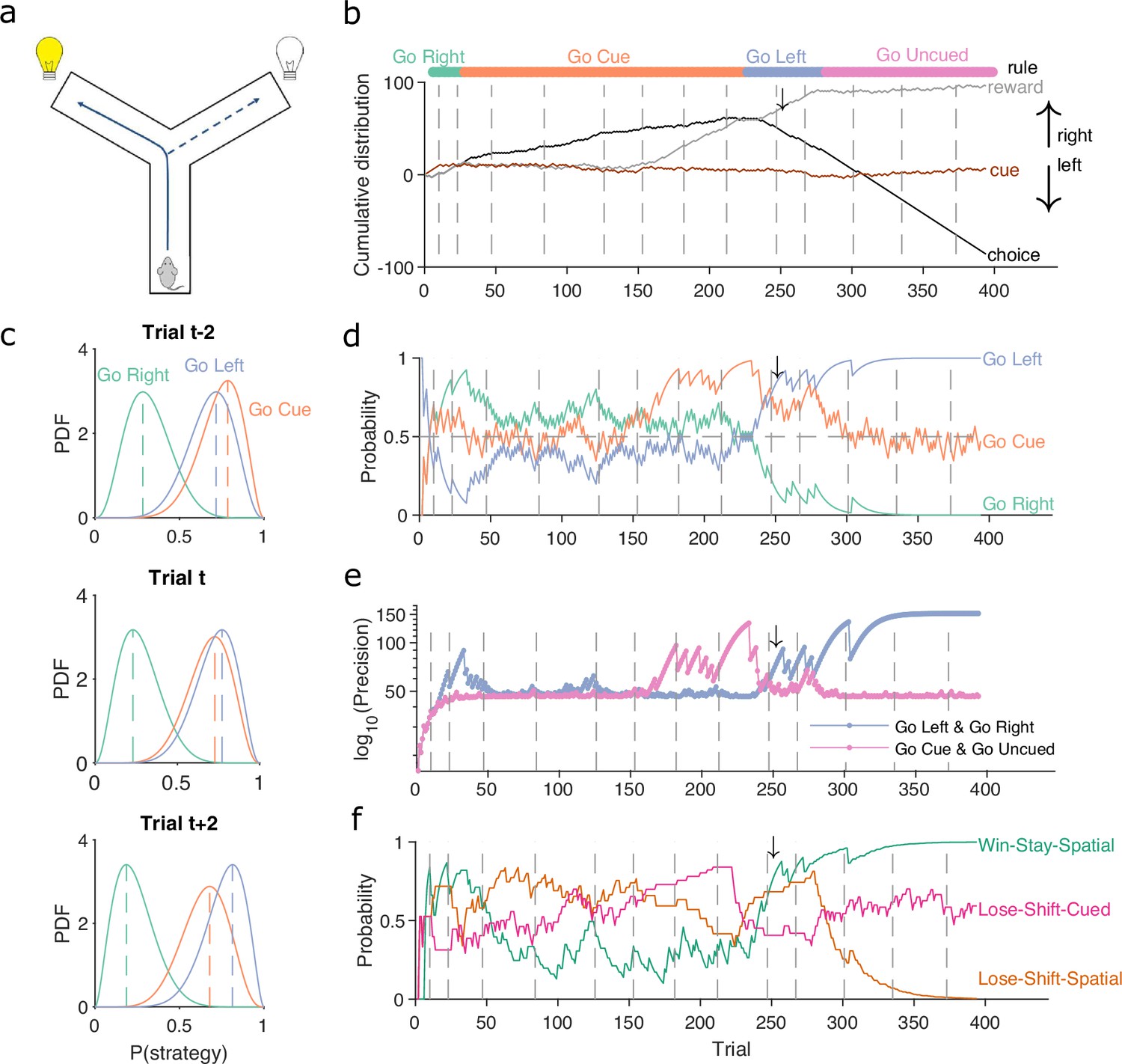
A Bayesian approach to tracking strategies.
(a) Schematic of the Y-maze task. The rat received a reward at the arm end if it chose the correct arm according to the currently enforced rule. A light cue was randomly switched on at the end of one of the two arms on each trial. Rules were in the sequence ‘go right’, ‘go cue’, ‘go left’, ‘go uncued’, and switched after 10 consecutive correct trials or 11 out of 12. (b) Example rat performance on the Y-maze task. We plot performance across 14 consecutive sessions: vertical grey dashed lines indicate session separation, while coloured bars at the top give the target rule in each trial. Performance is quantified by the cumulative distributions of obtained reward (grey) and arm choice (black). We also plot the cumulative cue location (brown), to show it is randomised effectively. Choice and cue distributions increase by +1 for right and decrease by −1 for left. Small black arrow indicates the trial t shown in panel c. (c) Example posterior distributions of three rule strategies for three sequential trials. Vertical dashed coloured lines identify the maximum a posteriori (MAP) probability estimate for each strategy. (d) Time-series of MAP probabilities on each trial for the three main rule strategies, for the same subject in panel b. Horizontal grey dashed line indicates chance. We omit ‘go uncued’ for clarity: as it is the complementary strategy of ‘go cue’ (P(go uncued) = 1 - P(go cued)), so it is below chance for almost all trials. (e) Precision (1/variance) for each trial and each of the tested strategies in panel d; note the precisions of mutually exclusive strategies (e.g. go left and go right) are identical by definition. (f) Time-series of MAP probabilities for three exploratory strategies. Staying or shifting is defined with respect to the choice of arm (Spatial) or the state of the light in the chosen arm (Cued) – for example if the rat initially chose the unlit arm and was unrewarded, then chose the lit arm on the next trial, this would be a successful occurrence of ‘Lose-Shift-Cued’.
Figure 1—figure supplement 1
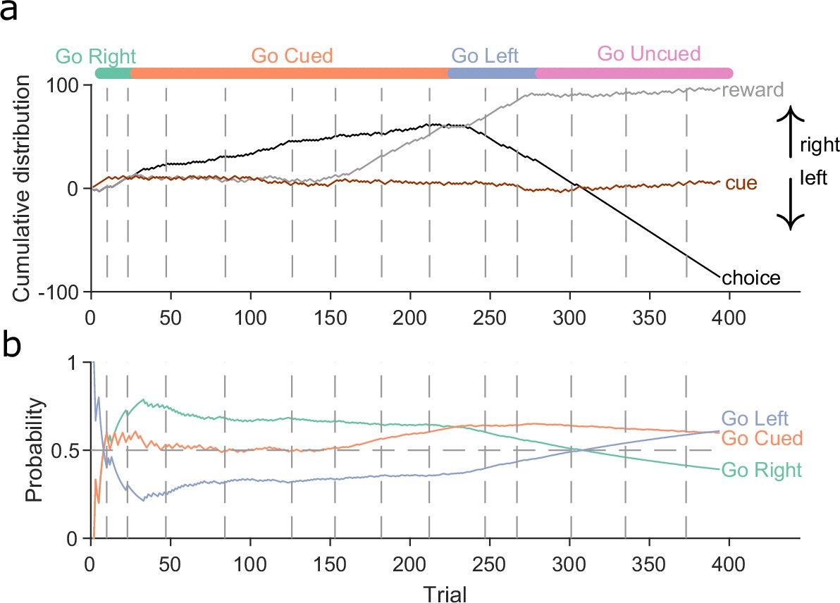
A stationary Bayesian approach fails to track behavioural changes.
(a) Same as Figure 1b. Example rat performance on the Y-maze task. Each curve shows the cumulative distribution of reward (grey), choice (black), and cue location (brown). Vertical grey dashed lines indicate sessions. Colours at the top indicate the target rule. (b) Maximum a posteriori (MAP) probabilities for three strategies across the 14 sessions for the example animal in panel a, when using Bayesian estimation without evidence decay. Note how the estimated probability of ‘go right’ remains the highest through both the switches to the ‘go cued’ and ‘go left’ rules, despite the animal clearly altering its behaviour, as it required 10 consecutive trials (or 11 out of 12) of the correct choice to switch the rule. Horizontal grey dashed line indicates chance level.
Figure 1—figure supplement 2
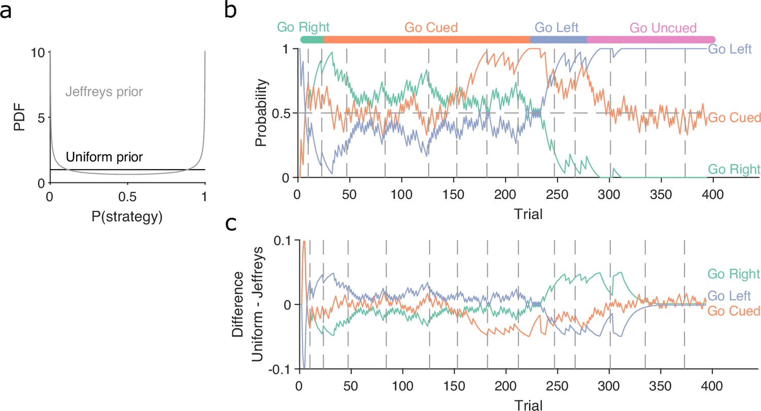
Robustness of the Bayesian approach to changes in the initial prior.
(a) Example of uniform and Jeffrey’s distributions used as the prior probability for the Bayesian algorithm. (b) Similar to Figure 1d, maximum a posteriori (MAP) probabilities over trials for the example rat in Figure 1b. The model is initialised with the Jeffrey’s prior. (c) Difference between the MAP probabilities for each strategy when initialised with either the uniform or the Jeffrey’s prior.
Figure 2 with 5 supplements
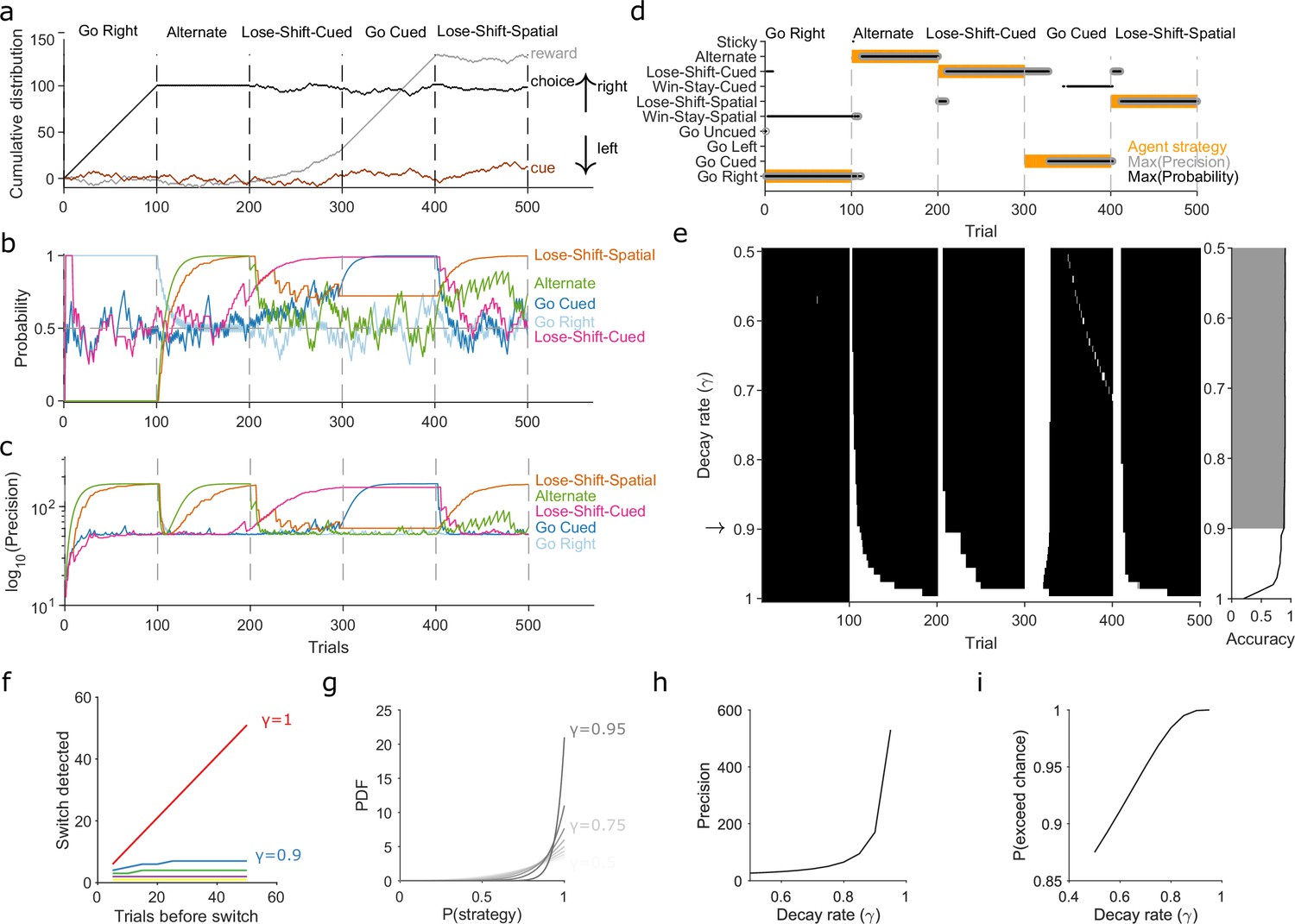
Robust tracking of strategies in synthetic data.
(a) Cumulative distribution of raw behavioural data for the synthetic agent, performing a two-alternative task of choosing the randomly cued option. Curves are as in Figure 1b. Vertical dashed lines indicate strategy switches by the agent. (b) Maximum a posteriori (MAP) values of for the five implanted strategies across trials, for . Chance is 0.5. (c) Precision for the five implanted strategies. (d) A decision rule to quantify the effect of . For every tested strategy, listed on the left, we plot for each trial the strategies with the maximum MAP probability (black dots) and maximum precision (grey circles) across all strategies, and the agent’s actual strategy (orange bars). Maximising both the MAP probability and precision uniquely identifies one tested strategy, which matches the agent’s strategy. (e) Algorithm performance across evidence decay rates. Left: successful inference (black) of the agent’s strategy using the decision rule. Right: proportion of trials with the correct detected strategy; grey shading shows values within the top 5%. Standard Bayesian inference is . (f) Number of trials until a strategy switch is detected, as a function of the number of trials using the first strategy. One line per decay rate (). Detection was the first trial for which the algorithm’s MAP probability estimate of the new strategy was greater than the MAP probability estimate of the first strategy. (g) The decay rate () sets an asymptotic limit on the posterior distribution of . We plot the posterior distribution here for an infinite run of successes in performing strategy i at a range of . (h) The asymptotic limits on the precision of the posterior distributions set by the choice of decay rate (). (i) The asymptotic limits on the probability that exceeds chance (p = 0.5) in a two-choice task.
Figure 2—figure supplement 1
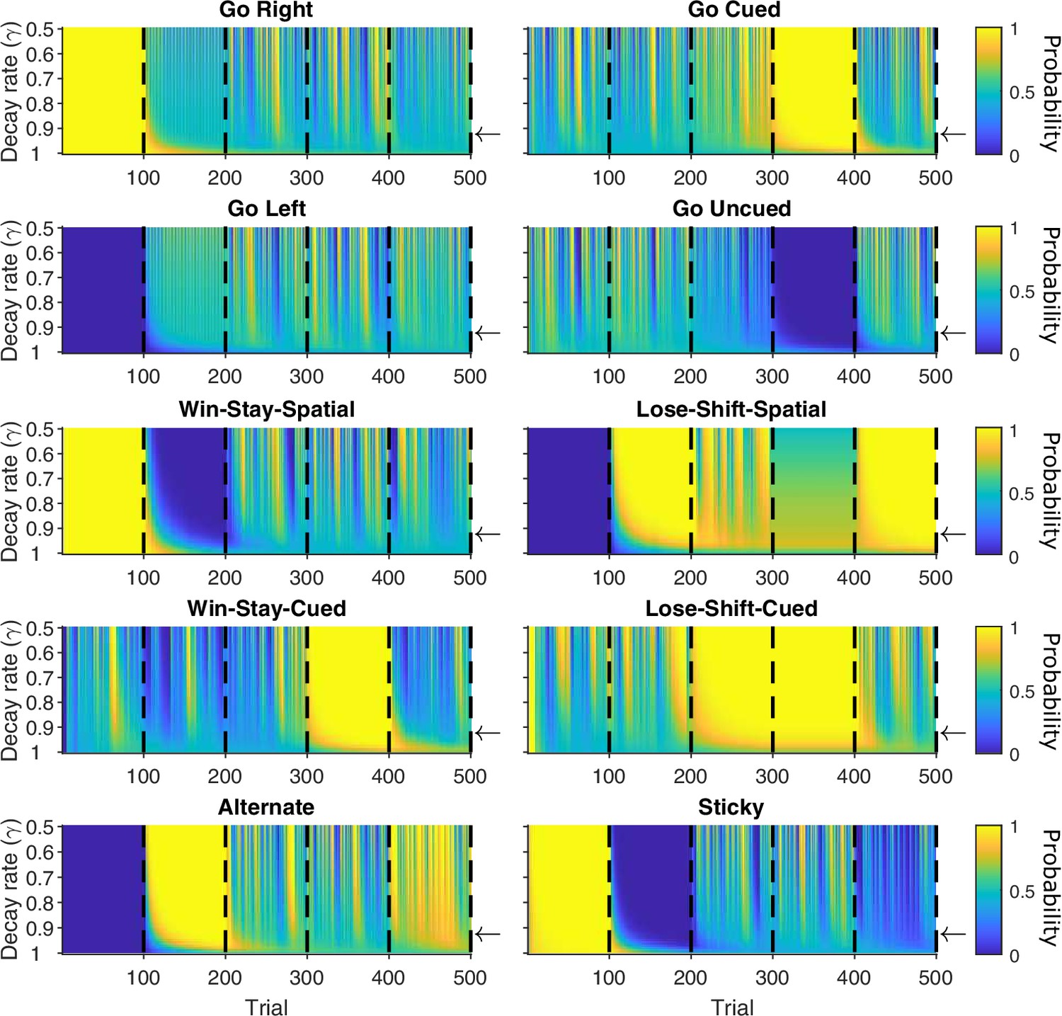
Maximum a posteriori (MAP) probabilities for agent strategies across changes in decay rate.
For the synthetic agent performing the five blocks of strategies, each panel plots the MAP values for one strategy, across each trial and each value of the decay rate between 0.5 and 1, in steps of 0.01. Vertical black dashed lines indicate block switches. Horizontal arrows are γ = 0.9.
Figure 2—figure supplement 2
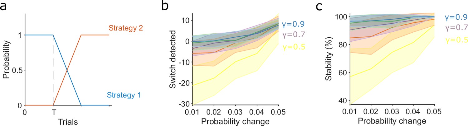
Slower evidence decay tracks gradual switches in strategy more accurately and robustly.
(a) Model for the gradual switch between two strategies after trial T . The probabilities of executing the two strategies change linearly at some rate m. Trial T is 500 in panels b and c, so that past-history effects have plateaued, giving worst-case performance for detection. Detection of the switch is measured from when the probabilities crossover: when the probability of executing strategy 2 exceeds that of executing strategy 1. (b) Accuracy of tracking gradual strategy switches increases with slower evidence decay. We plot the number of trials after the crossover trial until detection as a function of m, the rate of change in the execution probabilities. Negative values indicate detection before the crossover of probabilities; these false positive detections were due to a chance run of trials using the new strategy 2. Plots show means and standard deviation (SD) over 50 repeats; γ = 1 omitted as detection scales with T when there is no evidence decay. (c) Stability of the detected switch increases with slower evidence decay: the proportion of trials after the detection for which the algorithm reported the new strategy (strategy 2) was dominant. Plots show means and SD over 50 repeats.
Figure 2—figure supplement 3
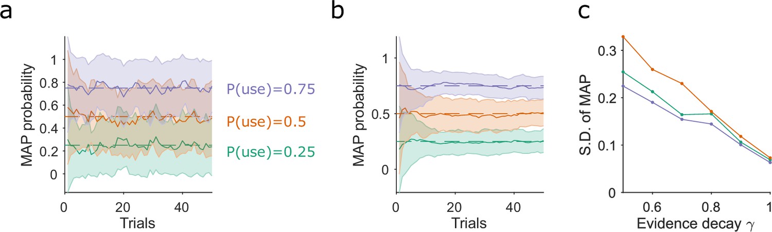
Slower evidence decay gives lower variability when tracking stochastic use of a strategy.
(a) Estimating the stochastic probability of using a strategy. For three different probabilities of using a strategy (p(use)), we plot the mean and standard deviation (S.D.) of the algorithm’s MAP estimate of that test strategy, over 50 simulations of 50 trials. Results shown for γ = 0.5. (b) As for (a), for γ = 0.9. (c) Variation in the MAP estimates of p(use) decreases with slower rates of evidence decay (higher γ). S.D. taken from trial 50 of 50 simulations similar to those in panels a and b.
Figure 2—figure supplement 4
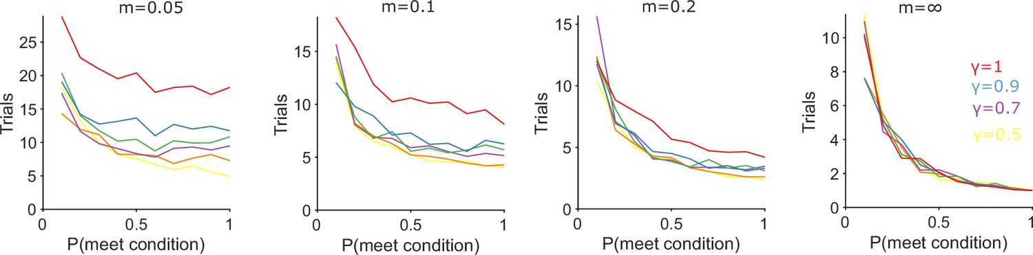
Algorithm performance for tracking a new conditional strategy.
Each panel plots the number of trials needed to track P(strategyi(t)|choices(1 : t)) above chance (0.5) after the appearance of a new conditional strategy whose condition occurs with probability p(meet condition). The probability of executing the new conditional strategy when its condition is met linearly increases from 0 to 1 with rate m. The right-most panel is the abrupt case (m = ∞) where the strategy’s probability is immediately 1.
Figure 2—figure supplement 5
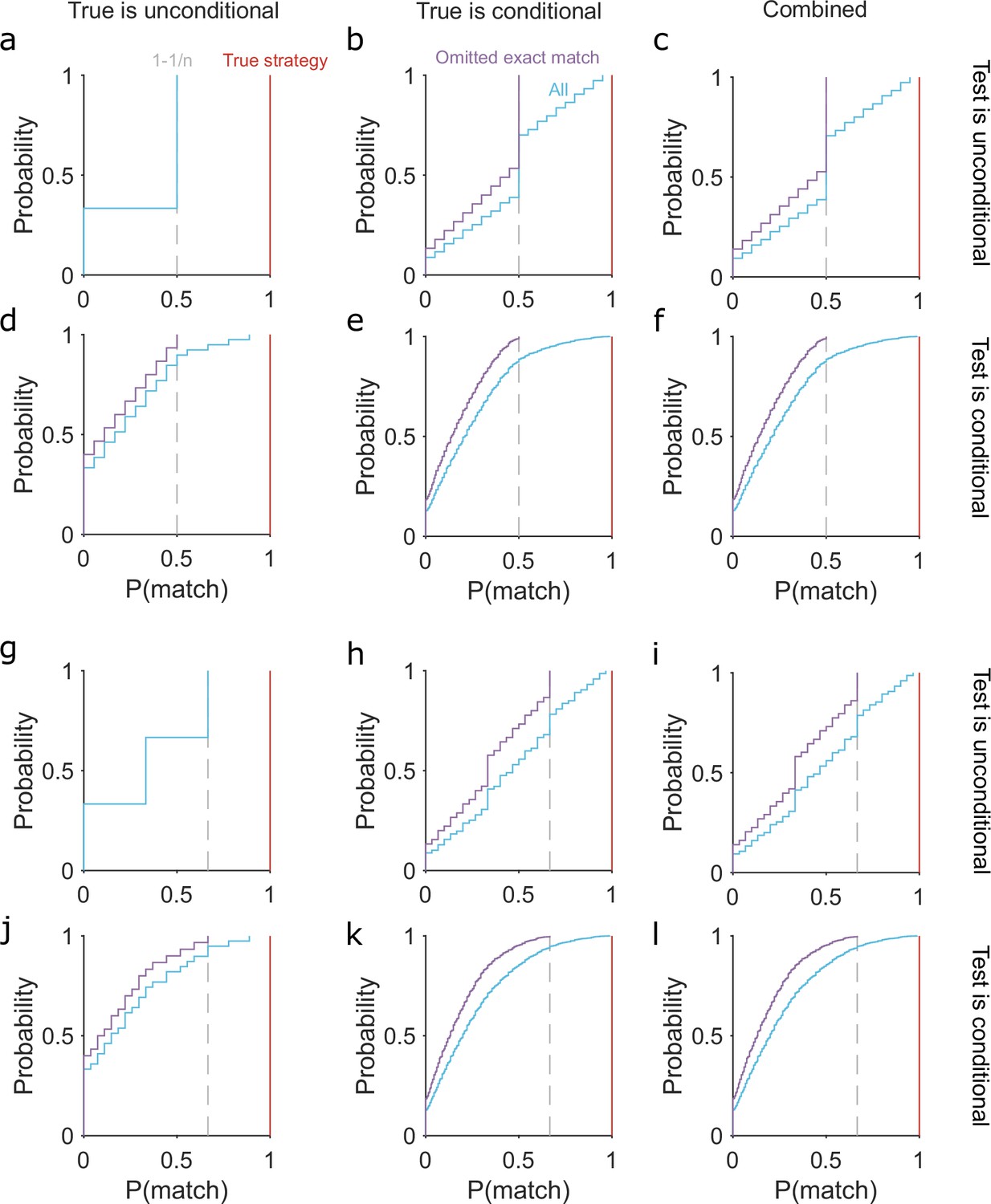
Limits on the probability of the tested strategy matching a true strategy used by an agent during exploration.
(a) The cumulative distribution of p(match) between the tested strategy and a true strategy when both are unconditional. For a task with n options p(match) can take one of three values: 0 (tested and true are mutually exclusive); 1/n (tested strategy chooses one option); 1 −1/n (the tested strategy chooses any but one option). (b) The distribution of p(match) when the tested strategy is unconditional, but one true strategy is conditional (blue: ‘All’). We evaluated p(match) using probabilities between 0.1 and 1 that this true strategy’s condition is met; and we allowed that the tested strategy could exactly match this true strategy either when the condition is met or when it is not. Not allowing this exact matching gives the distribution in purple, with a maximum at 1 − 1/n. (c) The full distribution of p(match) for when the tested strategy is unconditional, given by the combination of the relevant distributions in panels (a, b). Because we know the type of tested strategy, but not the type of true strategy used by a subject, these distributions place bounds on what we can infer from the maximum a posteriori (MAP) probability of a tested unconditional strategy. (d–f) As for (a–c), for when the tested strategy is conditional. (g–l) As for (a–f), for a task with n = 3 options. Note the maximum p(match) at 1 − 1/n (vertical dashed grey line) when the logical equivalence between tested and true strategies is omitted.
Figure 3 with 1 supplement
Detecting learning.
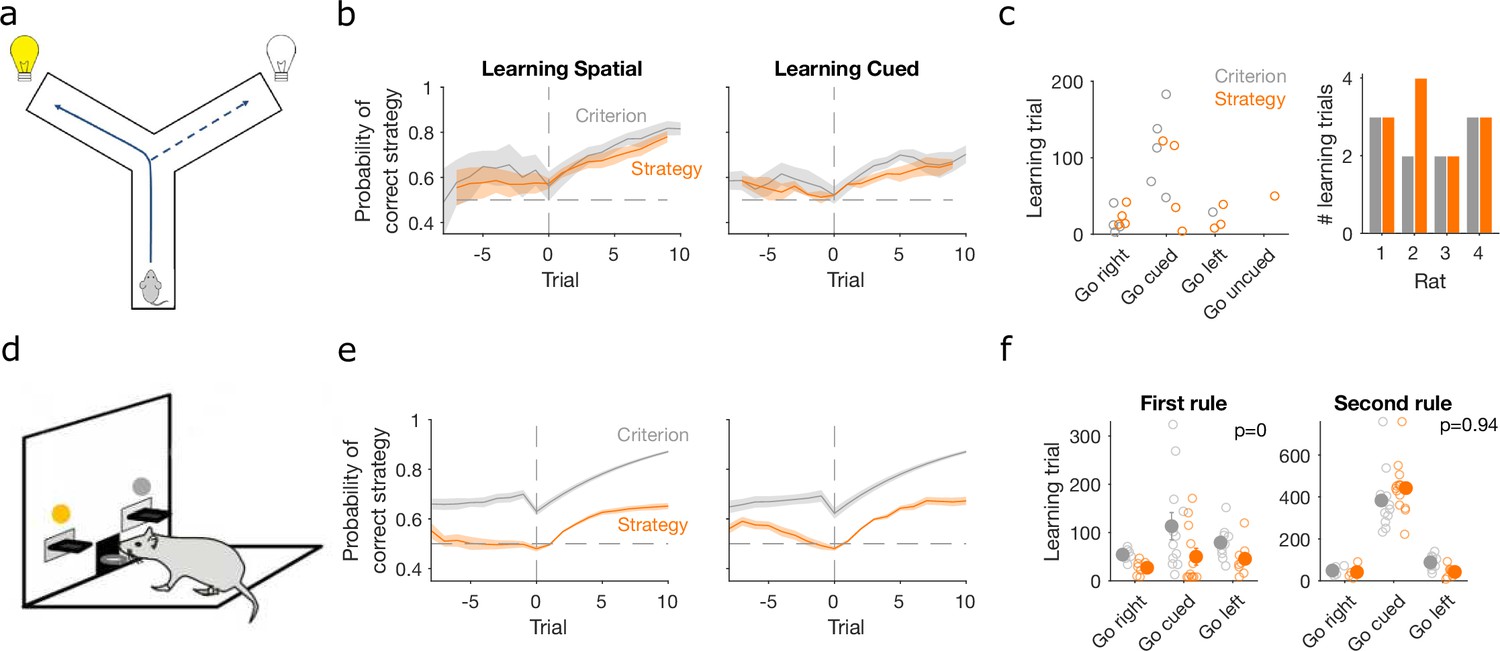
(a) Schematic of Y-maze task, from Figure 1a. (b) Maximum a posteriori (MAP) estimate of for the correct strategy for the spatial (left panel) and cued (right panel) rules on the Y-maze, aligned to the learning trial for each subject (trial 0, vertical dashed line). Learning trials are defined by the experimenters’ original criterion (grey) or by our strategy criterion (orange). Curves represent means (bold line) ± standard error of the mean (SEM; shading) for sessions meeting each criterion across the four rats (Spatial rule: original criterion , strategy criterion ; Cued rules: original criterion , strategy criterion ). Horizontal dashed line is chance. (c) Comparison between learning trials in the Y-maze task identified using the original criterion or our strategy criterion. Left: the identified learning trials for each rule. Trial zero was the first trial with that rule enforced, and rules are labelled in the order they were presented to the rats. Right: number of identified learning trials per rat. (d) Schematic of the lever-press task. Rats experienced both spatial (e.g. choose left lever) and cued (e.g. choose lit lever) rules. (e) As for panel b, for the lever-press task. rats. (f) Comparing the learning trials identified in the lever-press task by the original criterion or our strategy criterion for the first (left) and second (right) rule learnt by each rat. Solid symbols show mean and SEM; open symbols show individuals’ learning trials. p-values are from a Wilcoxon signed rank test between the learning trials identified by the original and by the strategy criterion ( rats). For the first rule, the learning trials based on the original and strategy criterion are 88.9 ± 12.3 and 59 ± 11.3 (mean ± SEM), respectively. For the second rule, the learning trials based on the original and strategy criterion are 224.3 ± 33 and 272 ± 33 (mean ± SEM), respectively. Note the second rule’s y-axis scale is a factor of 2 larger than for the first rule, because of the time taken to learn the cued rule second.
Figure 3—figure supplement 1
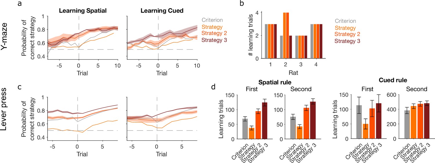
Performance of further learning criteria.
‘Criterion’ and ‘Strategy’ criteria are those shown in Figure 3 for classic trial-counting and maximum a posteriori (MAP) estimates contiguously above chance, respectively. We compare those here to two more stringent criteria: ‘Strategy 2’: the first trial at which the MAP estimate for the rule strategy is above chance and the precision of the posterior distribution is greater than all others; ‘Strategy 3’: the first trial at which the probability of the posterior distribution P(strategyi(t)|choices(1 : t)) containing chance fell below some threshold θ = 0.05. (a) For the Y-maze task, the MAP estimate of P(strategyi(t)|choices(1 : t)) for the target-rule strategy around learning defined by the four tested learning criteria. Lines represent means over sessions; shading shows standard error of the mean (SEM). (b) The number of learning trials per animal identified by each criterion. (c) As for panel a, for the lever-press task. (d) The identified learning trials in the lever-press task according to each criterion. The task had equal numbers of animals learn an egocentric or cued lever-press rule first, then switched to the other rule; the plots group animals by their experienced rule sequence. A three-factor analysis of variance (ANOVA) on criterion, rule type, and rule order confirmed a significant effect on learning trials of the choice of learning criterion (F = 8.91, p < 0.001); it confirmed that learning trials depended on rule type (F = 297.18, p < 0.001) and rule order (F = 270.12, p < 0.001); and it confirmed that the sequence of rules affected the speed of learning for all tested criteria, with cued rules taking substantially longer to learn after first learning a spatial rule (the interaction of rule order × rule type, F = 250.05, p < 0.001).
Figure 4
Detecting responses to task changes.
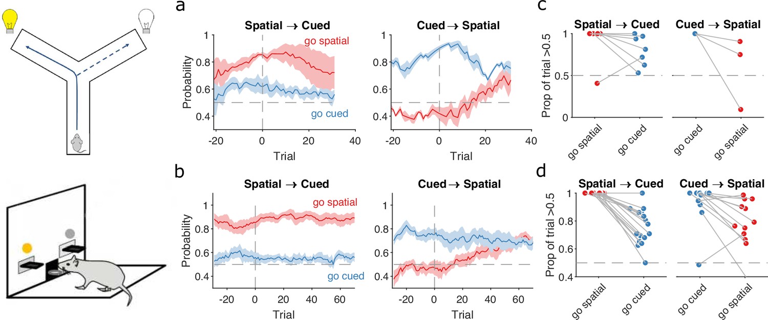
(a) Responses to rule switches in the Y-maze task. The left panel plots the maximum a posteriori (MAP) estimates of for the target spatial and cue strategies aligned to the switch from a spatial to a cued rule (N = 7 sessions, from four rats). The right panel plots the MAP estimates aligned to the switch from a cued to a spatial rule (N = 3 sessions, from three rats). For both panels, curves plot means ± standard error of the mean (SEM; shading) across sessions, aligned to the rule-switch trial (vertical dashed line). The horizontal dashed line indicates chance. (b) Same as panel a, but for the lever-press task. rats for spatial → cued; cued → spatial. (c) Response to each rule-switch in the Y-maze task. Each dot shows the proportion of trials after a rule switch in which the labelled strategy was above chance. Proportions calculated for a window of 30 trials after the rule switch. Lines join datapoints from the same switch occurrence. (d) Same as panel c, for the lever-press task. Proportions calculated for a window of 60 trials after the rule switch, to take advantage of the longer sessions in this task.
Figure 5
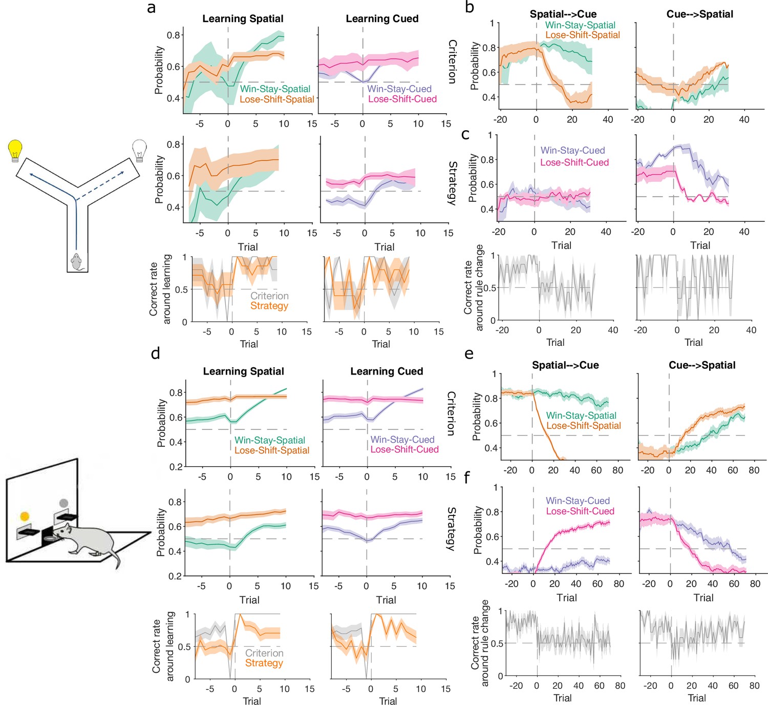
Lose-shift and win-stay independently change around learning and rule switches.
(a) Changes in the probability of win-stay and lose-shift strategies around learning. In the top pair of panels, we plot probabilities for choice-driven (left) and cue-driven (right) forms of win-stay and lose-shift aligned to the identified learning trial (trial 0). Learning trials identified by either the original study’s criterion (top) or our rule-strategy criterion (middle). The bottom panel plots the proportion of correct choices across animals on each trial. Lines and shading show means ± standard error of the mean (SEM; given in Figure 3b). (b) Rule switch aligned changes in probability for choice-based win-stay and lose-shift strategies ( given in Figure 4a). (c) Rule switch aligned changes in probability for cue-based win-stay and lose-shift strategies. (d–f) Same as panels a–c, but for the lever-press task. Panel d: rats per curve. Panels e, f: rats spatial → cued; cued → spatial.
Figure 6 with 1 supplement
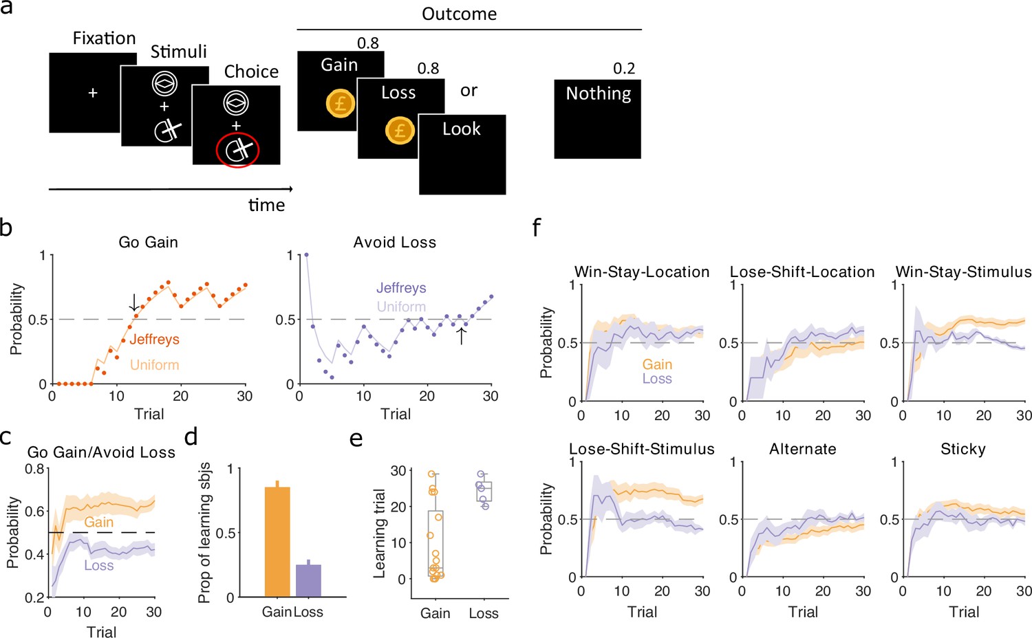
Human learning and exploration on a gain/loss task.
(a) Gain/loss task. Gain, loss, and look trials each used a different pair of stimuli and were interleaved. A pair of stimuli were randomly assigned to the top or bottom position on each trial. Numbers above Outcome panels refer to the probabilities of those outcomes in the gain and loss trial types. (b) For an example participant, the maximum a posteriori (MAP) estimate of for the target-rule strategy during gain (left panel) and loss (right panel) trials. We plot two estimates, initialised with our default uniform prior (solid) or Jeffrey’s prior (dotted). Horizontal dashed lines indicate chance level. Black arrows indicate the learning trial based on our strategy criterion. (c) The MAP estimate of for the target-rule strategies across all participants. Curves plot mean ± standard error of the mean (SEM) (shading) across 20 participants. The dashed line is chance. (d) Proportion of participants that learnt the target strategy for gain or loss trials. Learning was identified by the first trial at which the MAP estimate of was consistently above chance until the end of the task (black arrows in panel b). Vertical bar indicates the 95% Clopper–Pearson confidence intervals for binomial estimates. (e) Distributions of learning trials for gain and loss trials, for the participants meeting the learning criterion. Each dot is a subject. Boxplots show the median, and the 25th and 75th percentiles. The whiskers extend to the extreme values. (f) Probabilities of exploratory strategies for the learning participants (N = 13 for gain, N = 5 for loss). Curves plot mean ± SEM (shaded area) MAP probabilities.
Figure 6—figure supplement 1
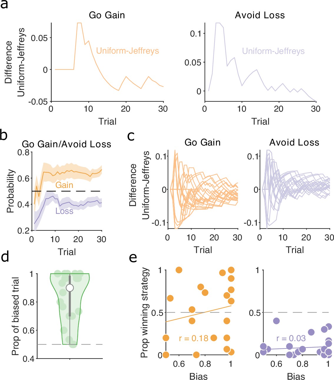
Human strategies are robust to priors and do not correlate with bias in preferred target locations.
(a) Difference between maximum a posteriori (MAP) probability of ‘go gain’ and ‘avoid loss’ strategies initialised with uniform prior and Jeffrey’s prior for the example participant in Figure 6b. (b) MAP probability profiles for ‘go gain’ and ‘avoid loss’ strategies along the session during gain and loss trials, respectively. Mean (solid curve) ± standard error of the mean (SEM; shaded area) across participants (N = 20). Horizontal dashed line indicates chance level. These strategies were initialised with Jeffrey’s prior. (c) Similar to panel a, the difference between the MAP probability of ‘go gain’ and ‘avoid loss’ strategies initialised with uniform and Jeffrey’s prior for every participant (one line per participant). (d) The distribution of biased trials during Look trials, defined as the proportion of trials in which the MAP probability for using a direction strategy towards one of the two stimulus locations was consistently above chance. No bias corresponds to 0.5, whereas 1 is when the participant chose the same location on every Look trial. Each dot is a participant. White dot is median and grey bars show the 25th and 75th percentiles. (e) The proportion of trials in which ‘go gain’ (left panel) and ‘avoid loss’ (right panel) were the winning strategy for each subject as function of their look bias. Each dot is a participant. r is the Pearson correlation coefficient. Solid line plots the linear fit to the data.
Figure 7
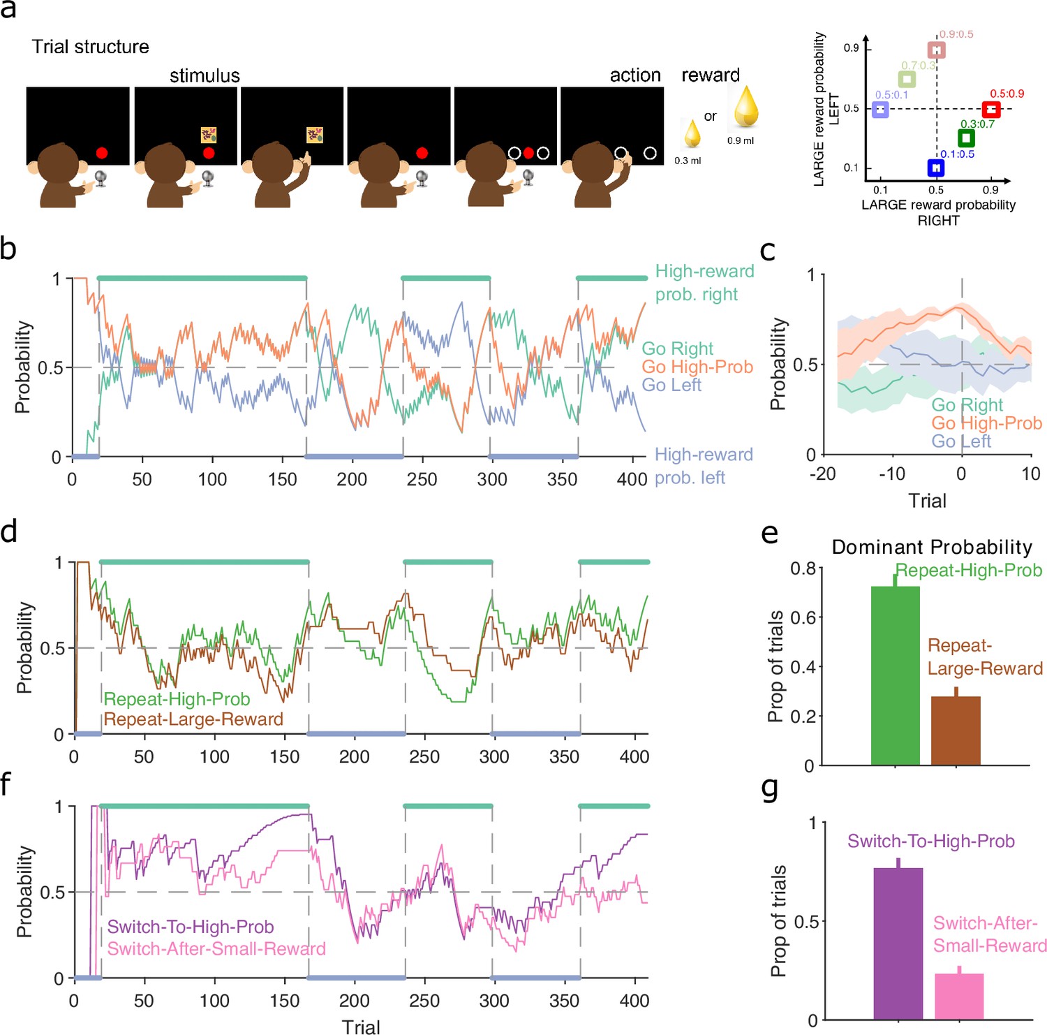
Probabilistic reward.
(a) Schematic of the stimulus-to-action reward task. Left: the monkey initiated a trial by touching a key after the red dot appeared on-screen. A stimulus appeared, predicting which side of the upcoming choice would have the higher probability of obtaining the large reward. Touching the stimulus and then the key brought up the choice options on-screen. The monkey indicated its decision by touching the appropriate circle on-screen. Right: probabilities of obtaining the large reward for each of the six stimuli. (b) Maximum a posteriori (MAP) probability for the strategy of choosing the side with the highest probability of reward (go high-probability side). We also plot the MAP probabilities for the choice of side (left or right). Green and blue dots at the top and bottom indicate the side with the higher probability of receiving the large reward; probabilities switched (vertical dashed lines) after the subject chose the high-probability option on 80% of trials in a moving window of 20 trials. (c) MAP probabilities in panel b aligned to the transition between blocks (trial 0). Average (bold lines; n = 5 blocks) ± standard error of the mean (SEM; shaded areas). (d) MAP probabilities along the session for exploratory strategies based on repeating the previous choice after either receiving the large reward or choosing the option with the higher probability of the large reward. (e) Proportion of trials in which the two repeating-choice strategies had the largest MAP probability. Vertical bars are 95% Clopper–Pearson confidence intervals. (f) As panel d, for exploratory strategies based on switching from the previous choice after either receiving the low reward or choosing the option with the lower probability of high reward. (g) As panel e, for the switching strategies in panel f.
Tables
Table 1
Rule strategy models for rat tasks.
Columns give the conditions to define trial as a success, failure, or null for each strategy corresponding to a target rule. The rule strategies we consider here do not have null conditions.
| Success | Failure | Null | |
|---|---|---|---|
| Go left | Chose left option | Did not choose left option | n/a |
| Go right | Chose the right-hand option | Did not choose the right-hand option | n/a |
| Go cued | Chose cued option (e.g. the lit lever) | Did not choose the cued option | n/a |
| Go uncued | Chose the uncued option (e.g. the unlit lever) | Did not choose the uncued option | n/a |
Table 2
Exploratory strategy models for rat tasks.
Columns give the conditions to define trial as a success, failure, or null for each exploratory strategy.
| Success | Failure | Null | |
|---|---|---|---|
| Win-stay-spatial | Rewarded on trial AND chose the same spatial option (e.g. the left lever) on trial | Rewarded on trial AND NOT chosen the same spatial option on trial | Unrewarded on trial |
| Lose-shift-spatial | Unrewarded on trial AND chose a different spatial option (e.g. the left lever) on trial | Unrewarded on trial AND NOT chosen a different spatial option on trial | Rewarded on trial |
| Win-stay-cue | Rewarded on trial AND chose the same cued option on trial (e.g. chose the lit lever on trials and ; or the unlit lever on trials and ) | Rewarded on trial AND NOT chosen the same cued option on trial | Unrewarded on trial |
| Lose-shift-cue | Unrewarded on trial AND chose a different cued option on trial from the choice on trial (e.g. chose the lit lever on trial and the unlit lever on trial ; or the unlit lever on trial and the lit lever on trial ) | Unrewarded on trial AND NOT chosen a different cued option on trial | Rewarded on trial |
| Alternate | Chose another spatial option compared to the previous trial | Chose the same spatial option as the previous trial | n/a |
| Sticky | Chose the same spatial option as the previous trial | Chose another spatial option compared to the previous trial | n/a |
Table 3
Exploratory strategy models for the non-human primate stimulus-to-action task.
Columns give the conditions to define trial as a success, failure, or null for each exploratory strategy.
| Success | Failure | Null | |
|---|---|---|---|
| Repeat-Large-Reward | Obtained the large reward on trial AND chose the same option on trial | Obtained the large reward on trial AND NOT chosen the same option on trial | Obtained the small reward on trial |
| Repeat-High-Prob | Chose the higher probability of large reward option on trial AND chose the same option on trial | Chose the higher probability of large reward option on trial AND NOT chosen the same option on trial | Chose the lower probability of large reward option on trial |
| Switch-After-Small-Reward | Obtained the small reward on trial AND NOT chosen the same option on trial | Obtained the small reward on trial AND chosen the same option on trial | Obtained the large reward on trial |
| Switch-To-High-Prob | Chose the lower probability of large reward option on trial AND NOT chosen the same option on trial | Chose the lower probability of large reward option on trial AND chose the same option on trial | Chose the higher probability of large reward option on trial |
Additional files
Download links
A two-part list of links to download the article, or parts of the article, in various formats.
Downloads (link to download the article as PDF)
Open citations (links to open the citations from this article in various online reference manager services)
Cite this article (links to download the citations from this article in formats compatible with various reference manager tools)
Tracking subjects’ strategies in behavioural choice experiments at trial resolution
eLife 13:e86491.
https://doi.org/10.7554/eLife.86491


