Figures and data in A theory of hippocampal theta correlations accounting for extrinsic and intrinsic sequences

Version of Record

The authors declare this version of their article to be the Version of Record.

About eLife's process

Download
Cite
Share
CommentOpen annotations (there are currently 0 annotations on this page).

Version of Record published: October 4, 2023 (This version)
Reviewed preprint version 3: September 18, 2023 (Go to version)
Reviewed preprint version 2: August 14, 2023 (Go to version)
Reviewed preprint version 1: May 17, 2023 (Go to version)
Sent for peer review: March 2, 2023
Preprint posted: February 5, 2023 (Go to version)

Figures
Tables
Additional files

8 figures, 2 tables and 1 additional file

Figures

Figure 1

Download asset Open asset

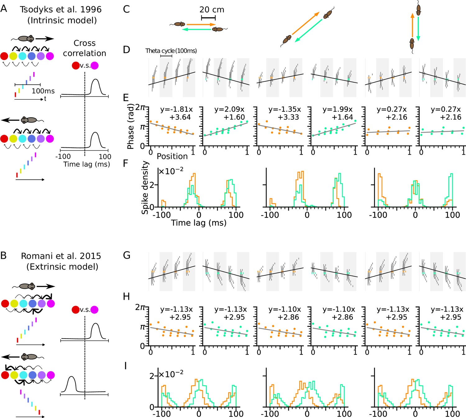
Phase precession depends on running direction in intrinsic models but not extrinsic models.

(A) Left: Schematic illustration of the intrinsic Tsodyks et al., 1996 model. When the animal runs through a series of place fields (solid circles) in 1-D, the place cells fire action potentials in sequence at the theta timescale (spike raster with corresponding colors). Recurrent connectivity is pre-configured and asymmetrical (connection strengths indicated by arrow sizes). Right: Cross-correlation function between the red and magenta cell, which remains the same for both running directions. (B) Left: Schematic illustration of the extrinsic Romani and Tsodyks, 2015 model. Recurrent connections behind the animal are temporarily depressed by short-term plasticity, and thereby, become movement-dependent. Right: Cross-correlation flips sign in the opposite running direction. (C) Simulated trajectories (duration 2 s) in a 2-d environment (80×80 cm) with speed 20 cm/s in left and right (left column), diagonal (middle), and up and down (right) directions. (**D–F**) Simulation results from the intrinsic model (with fixed asymmetrical connectivity inspired by the Tsodyks et al., 1996 model). Place cells only project synapses to their right neighbors. (D) Spike raster plots of place cells along the orange (left panel) and light green (right panel) trajectories (colors defined in C). Theta sequence order remains the same in the reversed running direction. Black line indicates animal position. (E) Phase-position relation for the spikes colored in C. Linear-circular regression (gray line) parameters are indicated on top. Positions of the animal at the first and last spike are normalized to 0 and 1, respectively. (F) Averaged cross-correlation of all cell pairs separated by 4 cm along the trajectory. Reversal of running direction does not flip the sign of the peak lags. (**G–I**) Same as D-F, but for the extrinsic model (spike-based variant of Romani and Tsodyks, 2015 model). Correlation peaks flip after reversal of running direction.

Figure 2

Download asset Open asset

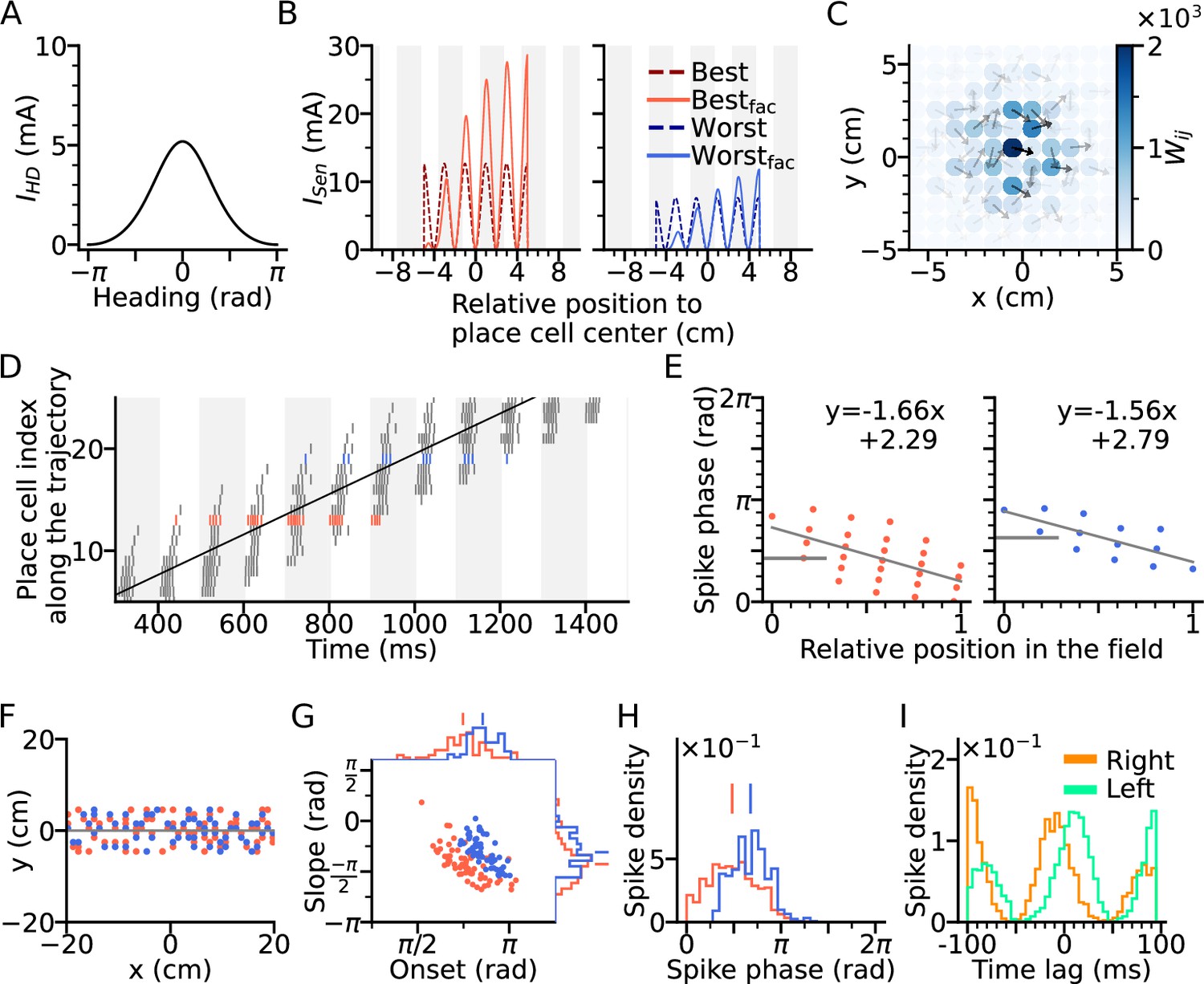
Directional input gives rise to spikes at lower theta phase.

(A) Directional input component of an example place cell. (B) Total sensory input as the sum of directional and positional drive of an example place cell for the animal running along (red dashed line, left) and opposite (blue dashed line, right) the preferred heading direction of the cell, respectively named as *best* and *worst* direction. The sensory input is modelled by oscillatory currents arriving with +70° phase shift relative to theta peaks (gray vertical lines). Place fields are defined by a 5 cm rectangular envelope. Solid lines depict the input current including short-term synaptic facilitation. (C) Synaptic weights ( $W_{i j}$ , color) from the place cell at the center (the darkest dot) to its neighbors in the 2-d environment. Each dot is a place field center in 2-d space. Arrows depict their preferred heading directions. (D) Spike raster plot sorted by visiting order of the place fields along the trajectory. Spikes of the cells with best and worst direction are colored in red and blue, respectively. (E) Phase position plots for the cells with best and worst direction from D (labels as in Figure 1E). The mean phase is marked as horizontal gray bar. (F) Example place cell centers with best (<30° different from the trajectory; red) and worst (>150°; blue) directions relative to the rightward trajectory (gray line). Only centers of cells that fire more than 5 spikes are shown. (G) Slopes and onsets of phase precession of the population from (F). Marginal slope and onset distributions are plotted on top and right, respectively. Note higher phase onset in the worst-direction case. (H) Spike phase distributions. Higher directional inputs generate lower spike phases. (I) Average spike correlation between all pairs with 4 cm of horizontal distance difference when the animal runs rightwards and leftwards. Peak lags are flipped as expected from an extrinsic model.

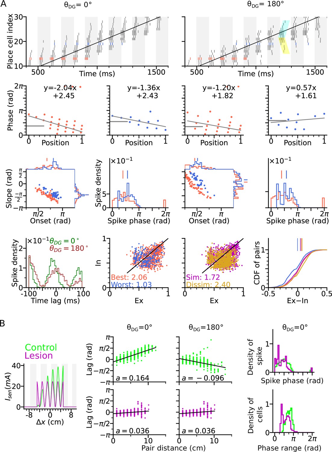
Figure 3 with 2 supplements

Download asset Open asset

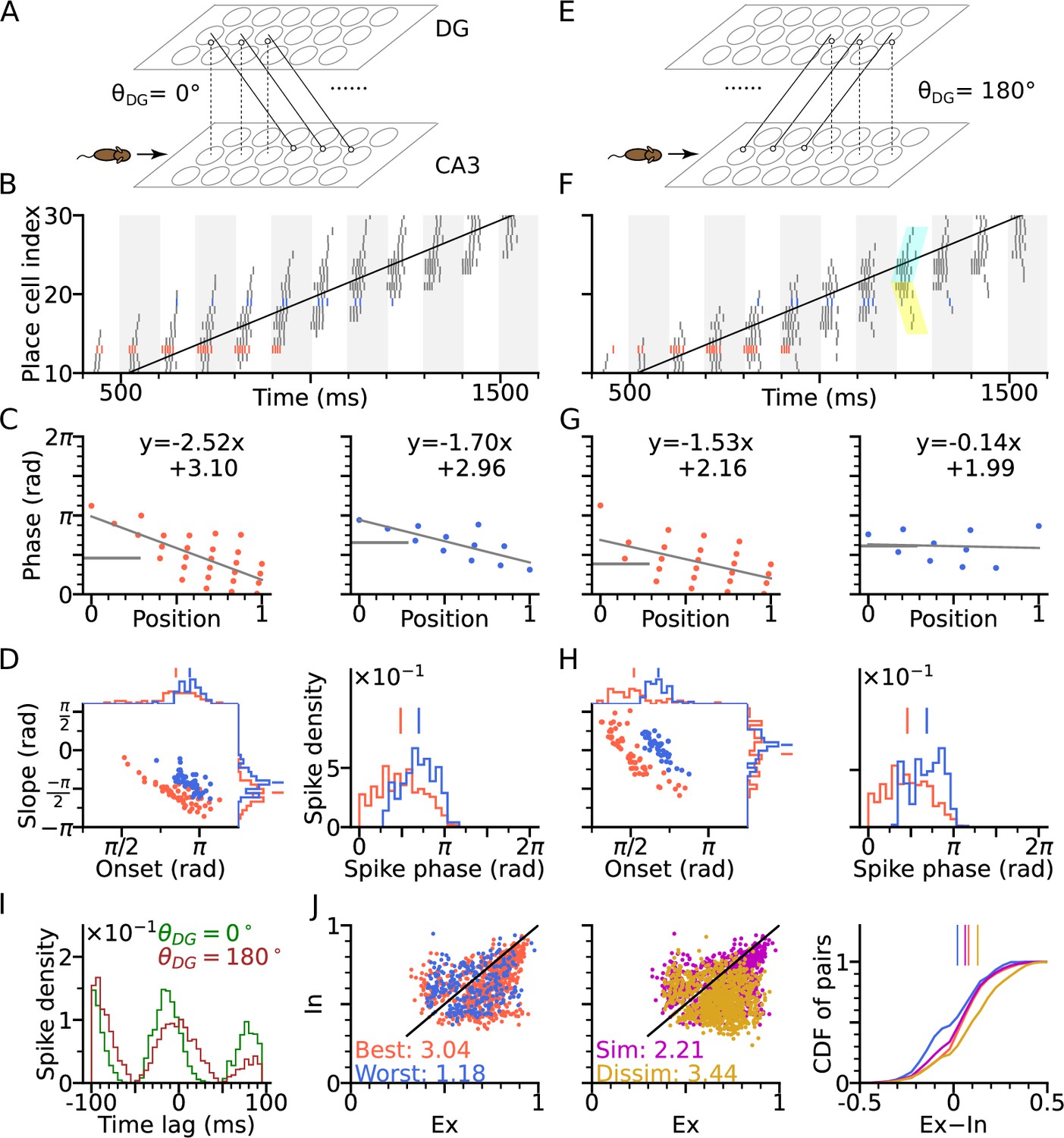
DG-CA3 loop introduces directionality of theta sequences.

(A) Illustration of synaptic connections from CA3 place cells to DG and vice versa. DG layer mirrors the place cell population in CA3 and redirects the CA3 inputs back to different locations. Here, DG cells project into CA3 place cells with fields 4 cm displaced to the right of the pre-synaptic CA3 cells. $θ_{DG}$ denotes the angular difference between the DG projection direction and the animal’s movement direction. (B) Spike raster plots sorted by cell indices along the trajectory (2 s duration) from x=-20 cm to x=20 cm. Cells with best and worst angles are marked by red and blue colors, respectively. (C) Phase-position plots as is Figure 2E. (D) Distributions of precession slopes, onsets and spike phases as in Figure 2G–H. (**E–H**) Same as A-D, but with DG cells projecting opposite to the animal’s movement direction ( $θ_{DG} = 180^{\circ}$ ). In F, cyan and yellow shaded regions indicate the examples of forward sequence induced by the movement (extrinsic), and backward sequence induced by the DG recurrence (intrinsic), respectively. (I) Average spike correlations for $θ_{DG} = 0^{\circ}$ and $θ_{DG} = 180^{\circ}$ for pairs separated by 4 cm along the trajectory. Note that for $θ_{DG} = 180^{\circ}$ , there is a relative excess of spike-pairs with positive lags. (J) Left: Intrinsicity and extrinsicity (see Methods) for all pairs from the populations with best (red) and worst (blue) direction. Pair correlations above and below the identity line are classified as intrinsic and extrinsic, respectively. Numbers are the ratios of extrinsically to intrinsically correlated field pairs. Note that the red best direction pairs are more extrinsic than the blue worst direction pairs due to higher sensory input. Middle: Ex/Intrinsicity of pairs with similar (<30°) and dissimilar (>150°) preferred heading angles. Pairs with similar preferred heading angle s are more intrinsic due to stronger DG-CA3 recurrence. Right: Cumulative distribution of the differences between extrinsicity and intrinsicity. Dissimilar and best direction pairs have higher bias to extrinsicity than similar and worst direction pairs, respectively.

Figure 3—figure supplement 1

Download asset Open asset

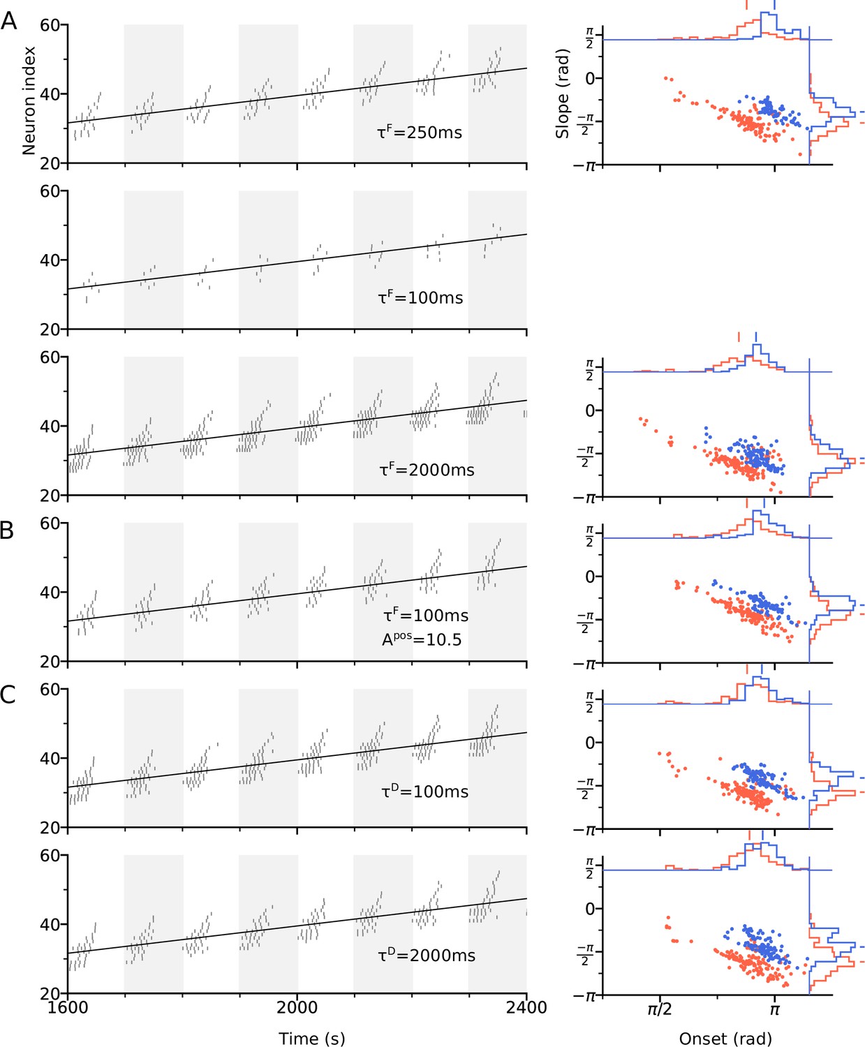
Effects of STF and STD time constants on theta sequences.

(A) Left: Spike raster plot of the CA3 place cells along the trajectory at = $τ^{F}$ 250ms (top row), 100ms (middle) and 2000ms (bottom). Conventions follow Figure 3B. Decreasing $τ^{F}$ allows faster recovery time of the sensory input to its resting value, $S_{0}^{F} = 0$ thus reducing the amount of depolarization and firing rate, as compared to = $τ^{F}$ 500ms used in Figure 3. However, the temporal order of theta sequences remains unchanged. Right: Distribution of slopes and onsets of phase precession in the best and worst directions, following the conventions of Figure 3D. At = $τ^{F}$ 100ms, the place cells do not generate enough spikes (spike count ≤ 5) for the analysis. (B) Increasing the amount of sensory input $A^{p o s}$ by 60% (from 6.5 in Figure 3 to 10.5 here) can restore the firing activity and theta sequences at $τ^{F}$ = 100ms. (C) Changing the STD time constant $τ^{D}$ does not noticeably affect the temporal structure of theta sequences and the distribution of phase precession slopes and onsets.

Figure 3—figure supplement 2

Download asset Open asset

Effects of running speed on theta sequences.

(A) Left: Spike raster plot of the CA3 place cells along the trajectory at running speed v=20 cm/s (top row), 40cm/s (middle) and 100cm/s (bottom). Conventions follow Figure 3B. As place cells are traversed at increasing velocities, their firing rate decreases due to insufficient depolarization. Right: Distribution of slopes and onsets of phase precession in the best and worst directions, following the conventions of Figure 3D. Only the distribution for running speed at 20 cm/s is shown. At running speed 40 cm/s and 100 cm/s, the place cells do not generate enough spikes (spike count ≤ 5) for the analysis. (B) Theta sequences at high running speed (100 cm/s) could be produced by a larger place field size (width of box-shaped input is increased to 15 cm compared to 5 cm in Figure 3) and longer DG projection ( $| r |$ =12 cm compared to 4 cm in Figure 3). Phase precession slopes and onsets are lower than in (A). (C) Increasing theta frequency to 12 Hz can recover the decrease of phase precession slope and onset from the high running speed (Rivas et al., 1996; Maurer et al., 2005). Model parameters are the same as Figure 3 in the main text unless specified at the bottom right of the raster plots.

Figure 4

Download asset Open asset

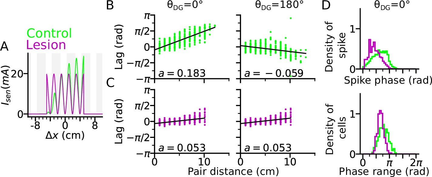
DG lesion reduces theta compression and phase precession range.

DG recurrence is turned off to simulate the lesion condition. (A) Positional sensory inputs into a place cell in lesion (purple) and control (green) cases. The control case is identical to Figure 3. In the lesion case, DG input is compensated by increased sensory input with increased probability of synaptic release, hence reduced short-term synaptic facilitation. (B) Theta compression, that is correlation between peak correlation lag and distance of field centers in the control case. Each dot represents a field pair. Linear-circular regression line is indicated in black. Note that the sign of regression slope ( $a$ in radians/cm) is determined by the directions of DG loop (negative in $θ_{DG} = 180^{\circ}$ ). (C) same as B, but for the lesion case. Theta compression is reduced as compared to the control condition. (D) Top: Distribution of spike phase during phase precession in all active (spike count > 5) cells in control and lesion case. Bottom: Distribution of phase precession range for all active cells.

Figure 5

Download asset Open asset

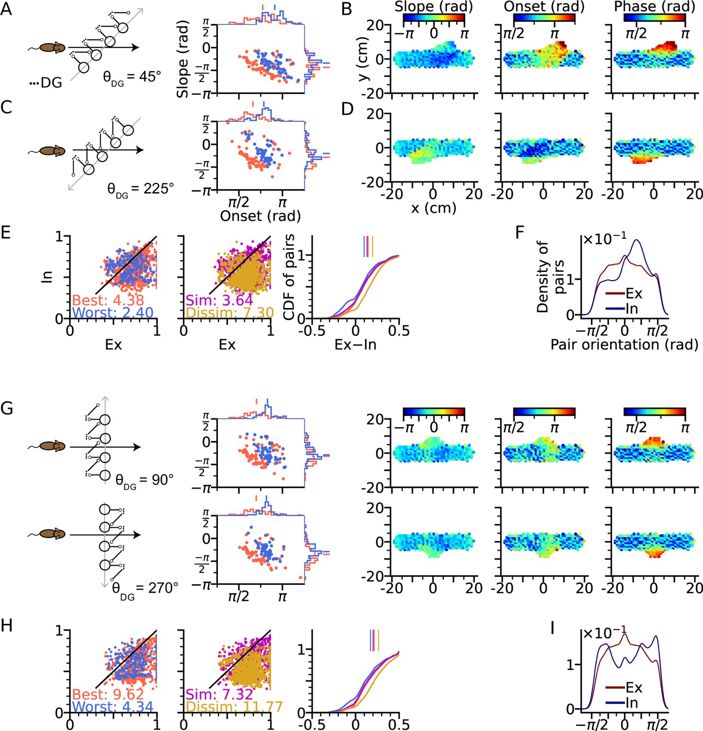
Intrinsic sequences lead to direction dependent 2-d phase precession and out-of-field firing (A) Left: Schematic illustration of DG-loop projection being tilted by 45° relative to the trajectory.

Right: Distributions of phase precession onsets and slopes from the place cells along the trajectory as in Figure 2G. (B) Slopes (left), onsets (middle) and mean spike phases (right) of phase precession from the place cells as a function of field center. High spike phases and onsets occur along the DG-loop orientation where intrinsic spiking dominates and yield out-of-field firing (see the extrusions from horizontal dot clouds) with late onsets and phases. (**C–D**) Same as A-B, but DG-loop projection is at 225° relative to trajectory direction. (D) For DG loops pointing opposite to the sensorimotor drive, prospective firing along the DG loop yields less steep precession slopes and lower onset. (E) Extrinsicity and intrinsicity of all place field pairs along the trajectory as in Figure 3J. Some pairs are totally extrinsic (Ex = 1) because DG projection is absent at those parts of the trajectory. (F) Density of field pairs with extrinsic/intrinsic correlation as a function of the orientation of field center difference vector relative to the x axis. Intrinsic fields peak at 45°. (G) Same as A-D, but DG-loop orientations are perpendicular to the trajectory direction at 90° (top) and 270°. Prospective spikes from intrinsic sequences are initiated in the perpendicular directions. (H) Same as E, but with higher Ex-In ratios. (I) Field pairs with intrinsic correlations are at ±90°.

Figure 6

Download asset Open asset

Extrinsically driven theta correlations can be temporally organized by sensorimotor drive alone without CA3-CA3 recurrence.

Simulations were performed without CA3-CA3 recurrence but with stronger spatial input. (A) Same as Figure 3. Extrinsically driven theta correlations and phase precession are still present. (B) Same as Figure 4. DG is still integral to the theta compression in a network model without CA3-CA3 recurrence.

Figure 7 with 1 supplement

Download asset Open asset

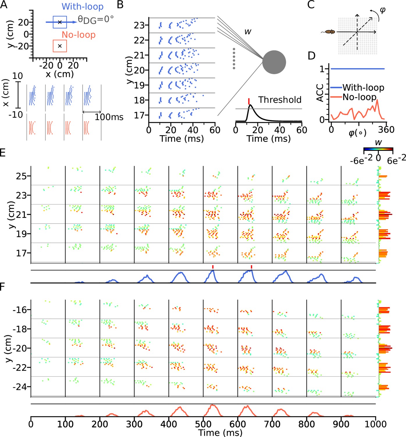
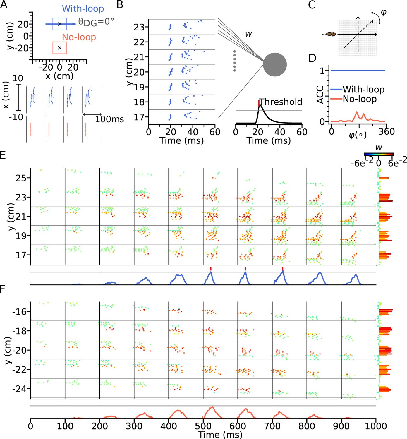
Intrinsic sequences provide a stable landmark for positional decoding using a tempotron.

(A) Top: Two tempotrons are trained for place cell populations within the top (with DG loop; blue) and bottom (no DG loop; red) squares, to recognize the presence of the corresponding sequence activities. DG-loop rightward projection is indicated by blue arrow and only exists in the blue square. Non-moving spatial inputs are applied to the CA3 network centered at the two locations (marked by black crosses) to evoke spike sequences for training. Bottom: Resulting spikes of the place cell network zoomed in to the subset of field centers from x=-10 to x=10 for y=+20 (with-loop, top raster plot) and y=-20 (no-loop, bottom). Each theta cycle is one (+) training pattern, which the tempotron is trained to detect by eliciting a spike. (B) Example training pattern with spikes of place cells from x=-10 to x=10 (in each rectangular row) fixed at different values of y. Only one theta cycle is shown. Each place cell delivers spikes to the dendrite of the tempotron, producing post-synaptic potentials (PSPs) at the soma (line plot at the bottom). Synaptic weights are adapted by the tempotron learning rule such that PSPs can cross the threshold (gray line) and fire for the detection of the sequence. After the tempotron has fired, the PSPs will be shunted. (C) Sequence detection is tested while the simulated animal ran on a trajectory with varying direction ( $φ$ ) from 0° to 360° with a 15° increment to detect the presence of the sequence. (D) Detection accuracies (ACC) for with-loop (red line) and no-loop (blue) input populations. Note that the tempotron cannot detect the no-loop sequences when tested on trajectories at various angles. (E) Detection of the intrinsic sequence for a trajectory $φ = 180^{\circ}$ for the DG-loop condition. Spike raster is shown for every two horizontal rows of place cells in the arena and color-coded by the synaptic weights (see color bar on the right). Tempotron soma potential is shown at the bottom for each pattern. (F) Same as E, but for no-loop inputs. The tempotron remains silent.

Figure 7—figure supplement 1

Download asset Open asset

Decoding of positional landmarks using tempotrons in a network model without CA3-CA3 recurrence.

Figure labels are the same as in Figure 7. Compared to the parameters in Figure 7, here CA3-CA3 weights were disabled ( $B^{dir} = 0$ ), but spatial input was increased during testing ( $A^{dir} = 14$ ,, $S_{0}^{F} = 0.25$ $S_{1}^{F} = 1.5$ ) and DG-loop strengths were increased ( $B^{DG} = 5500$ ).

Figure 8

Download asset Open asset

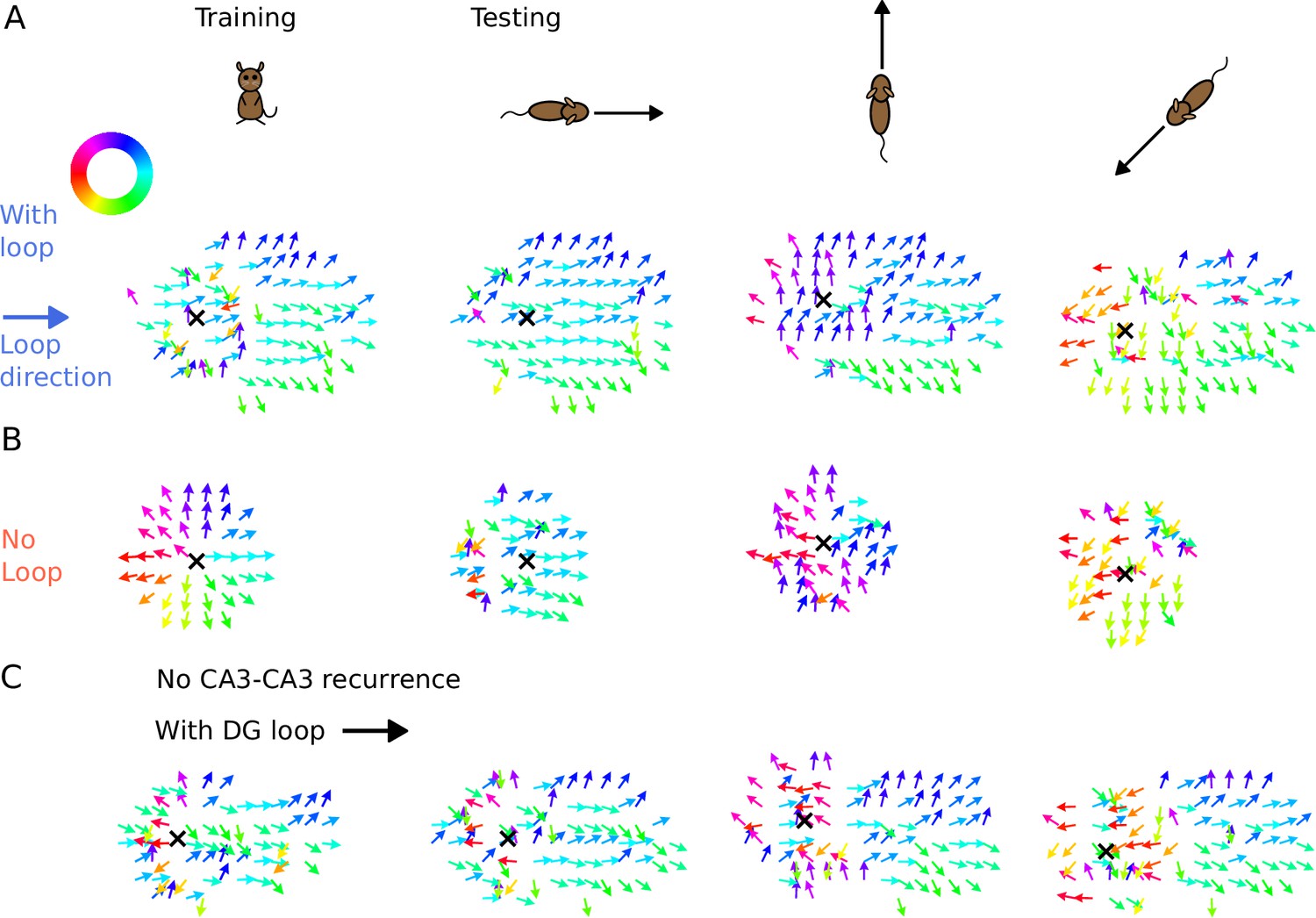
Illustration of spike time gradients in one theta cycle (500–600 ms) with and without DG loop.

(A) Time gradients with a DG loop projecting to the rightward direction ( $θ_{D G} = 0^{\circ}$ ). Each arrow is located at a CA3 place field center. The arrow direction indicates the spike time gradient, equivalently the ‘travelling direction’ of sequence activity, which is calculated as the sum of the directions to the 8 neighbouring field centers, weighted by the difference between their mean spike times in one theta cycle. Arrow direction is color-coded according to the color wheel. Black cross marks the instantaneous position of the animal. The first column shows the training condition when a non-moving spatial stimulus is applied. The three columns on the right show the testing condition when the rat is running in various directions. The sequence mostly propagates rightwards, following the DG-loop direction even when the animal runs in different directions. (B) Same as A without a DG loop. Sequences propagate outward from the animal position as a concentric travelling wave during training. During testing, spike time gradients follow the running direction. (C) Same as A, using the network model without CA3 recurrence. As in Figure 6, the extrinsic sequence is driven solely by the STF mechanism of the spatial input. Intrinsic sequences in this model still remain invariant to running directions and function as spatial landmarks.

Tables

Key resources table

Reagent type (species) or resource	Designation	Source or reference	Identifiers	Additional information
Software, algorithm	Python	Python Software Foundation	https://www.python.org/ RRID:SCR_008394
Software, algorithm	Linear-circular regression	Kempter et al., 2012		The algorithm is customized to our analyses
Software, algorithm	Tempotron	Gütig and Sompolinsky, 2006		The algorithm is customized to our analyses

Table 1

Model parameters used in simulations according to Figure panels.

In, Ex, C. and L. refer to intrinsic, extrinsic, control and lesion respectively.

Name \Figure	1 (In)	1 (Ex)	2	3	4 (L.)	5	6A	6B (C.)	6B (L.)	7
$A^{pos}$	7.5	9.0	6.5				9.5	7.5		6.5
$A^{dir}$	0		6				9	8		6
$S_{0}^{F}$	1		0		1.25	0	0.25	0	1.25	0
$S_{1}^{F}$	1		2		1.25	2	1.5	2	1.25	2
$Φ^{F}$	0		0.001		0	0.001			0	0.001
$B^{pos}$	1100		0
$B^{dir}$	0		2000	1500		2000	0			1500
$K^{CA3}$	0		1
$J_{i j}$	ON	OFF
$U^{D}$	0	0.9	0.7
$N_{DG}$	0			40×40 = 1600
$B^{DG}$	0			3000	0	4000		4000	0	4000
$K^{DG}$	0			1
$N_{I}$	0		250
$W_{0}^{CA3 - Inh}$	0		50
$W_{0}^{Inh - CA3}$	0		5
$W_{0}^{DG - Inh}$	0			350
$W_{0}^{Inh - DG}$	0			35

Additional files

MDAR checklist: https://cdn.elifesciences.org/articles/86837/elife-86837-mdarchecklist1-v1.pdf
Download elife-86837-mdarchecklist1-v1.pdf

Download links

A two-part list of links to download the article, or parts of the article, in various formats.

Downloads (link to download the article as PDF)

Open citations (links to open the citations from this article in various online reference manager services)

Mendeley

Cite this article (links to download the citations from this article in formats compatible with various reference manager tools)

Yuk-Hoi Yiu
Christian Leibold

(2023)

A theory of hippocampal theta correlations accounting for extrinsic and intrinsic sequences

eLife 12:RP86837.

https://doi.org/10.7554/eLife.86837.4

Share this article

Cite this article

Phase precession depends on running direction in intrinsic models but not extrinsic models.

Directional input gives rise to spikes at lower theta phase.

DG-CA3 loop introduces directionality of theta sequences.

Effects of STF and STD time constants on theta sequences.

Effects of running speed on theta sequences.

DG lesion reduces theta compression and phase precession range.

Intrinsic sequences lead to direction dependent 2-d phase precession and out-of-field firing (A) Left: Schematic illustration of DG-loop projection being tilted by 45° relative to the trajectory.

Extrinsically driven theta correlations can be temporally organized by sensorimotor drive alone without CA3-CA3 recurrence.

Intrinsic sequences provide a stable landmark for positional decoding using a tempotron.

Decoding of positional landmarks using tempotrons in a network model without CA3-CA3 recurrence.

Illustration of spike time gradients in one theta cycle (500–600 ms) with and without DG loop.

Model parameters used in simulations according to Figure panels.

MDAR checklist

Downloads (link to download the article as PDF)

Open citations (links to open the citations from this article in various online reference manager services)

Cite this article (links to download the citations from this article in formats compatible with various reference manager tools)