Uncovering circuit mechanisms of current sinks and sources with biophysical simulations of primary visual cortex
- Department of Informatics, University of Oslo, Norway
- Department of Physics, University of Oslo, Norway
- Department of Data Science, Norwegian University of Life Sciences, Norway
- MindScope Program, Allen Institute, United States
- Department of Physics, Norwegian University of Life Sciences, Norway
Figures
Figure 1
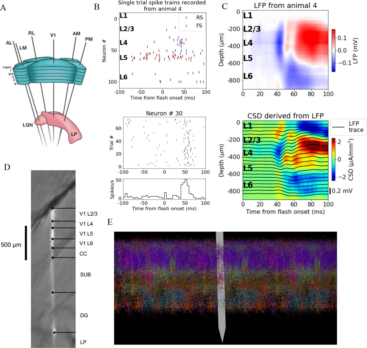
Illustration of experimental data and the biophysical model for mouse primary visual cortex (V1).
(A) Schematic of the experimental setup, with six Neuropixels probes inserted into six cortical (V1, latero-medial [LM], rostro-lateral [RL], antero-lateral [AL], postero-medial [PM], AM) and two thalamic areas (LGN, LP). (B) Top: spikes from many simultaneously recorded neurons in V1 during a single trial. Bottom: spikes from a single neuron recorded across multiple trials. In both cases, the stimulus was a full-field bright flash (onset at time 0, offset at 250 ms). (C) Top: local field potential (LFP) across all layers of V1 in response to the full-field bright flash, averaged over 75 trials in a single animal. Bottom: current source density (CSD) computed from the LFP with the delta iCSD method. (D) Histology displaying trace of the Neuropixels probe across layers in V1, subiculum (SUB) and dentate gyrus (DG). (E) Visualization of the V1 model with the Neuropixels probe in situ. (Image made using VND.)
Figure 2 with 3 supplements
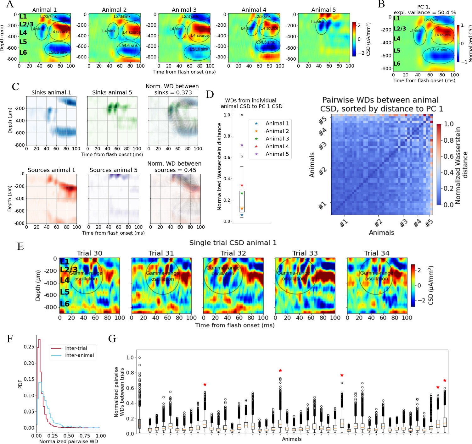
Variability in experimentally recorded current source density (CSD).
(A) Evoked CSD response to a full-field flash averaged over 75 trials, from five animals in the dataset. (B) The first principal component (PC) computed from the CSD of all n = 44 animals, explaining 50.4% of the variance. (C) Illustration of movement of sinks and sources in the calculation of the Wasserstein distance (WD) between the CSD of two animals in the dataset. The gray lines in the rightmost panels display how the sinks or sources of one animal are moved to match the distribution of sinks or sources of the other animal. (D) Left: WDs from each animal to the PC 1 CSD. Right: pairwise WDs between all 44 animals sorted by their distance to the first PC. (E) CSD from five individual trials in example animal 1. (F) Distribution of pairwise distances between single-trial CSD (red) and pairwise distances between trial-averaged CSD of individual animals (blue). Both are normalized to the maximum pairwise distance between the trial-averaged CSD of individual animals. (G) Pairwise WDs between trials in each of 44 animals (white boxplots), normalized to maximal pairwise WDs between trial-averaged CSD of animals. Gray-colored boxplot shows the distribution of pairwise WDs between trial-averaged CSD of individual animals, and the red stars indicate the n = 5 animals for which the inter-trial variability was greater than the inter-animal variability (assessed with Kolmogorov–Smirnov [KS] tests, p < 0.001 in all cases, see Figure 2—figure supplement 3).
Figure 2—figure supplement 1
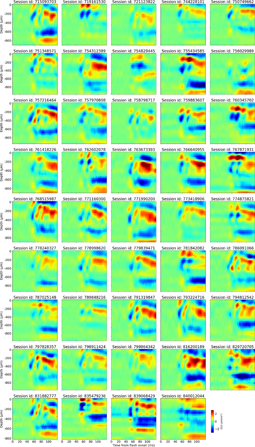
Trial-averaged current source density (CSD) during presentation of full-field flashes for all 44 animals in this study.
Figure 2—figure supplement 2

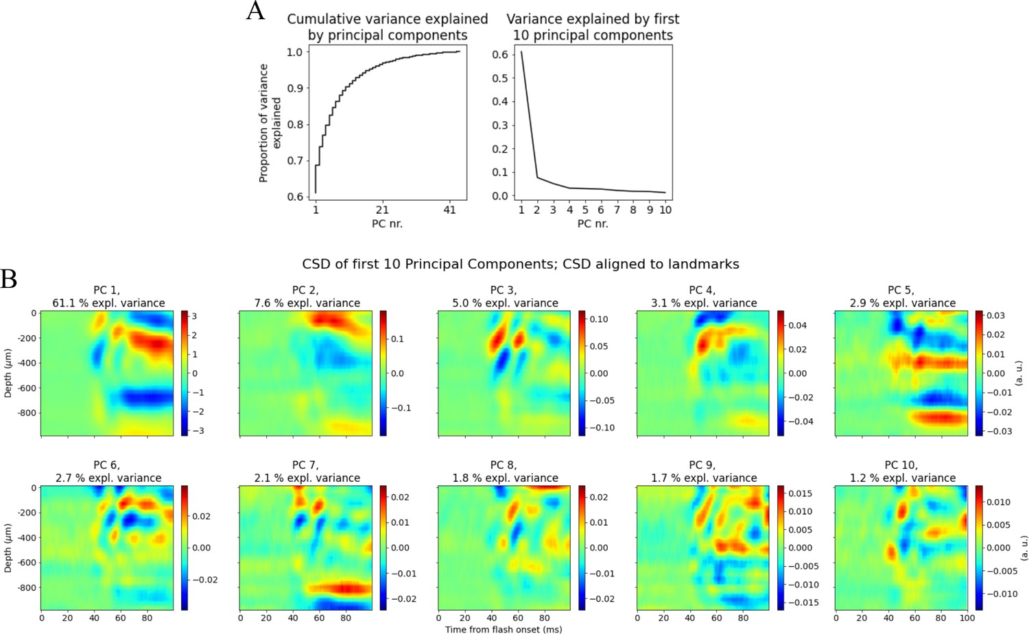
Principal component analysis (PCA) on histology-aligned current source density (CSD).
(A) Left: cumulative variance explained by principal components. Right: variance explained by first 10 components. (B) CSD plots of the first 10 principal components explaining in total >90% of the variance in trial-averaged CSD across animals.
Figure 2—figure supplement 3
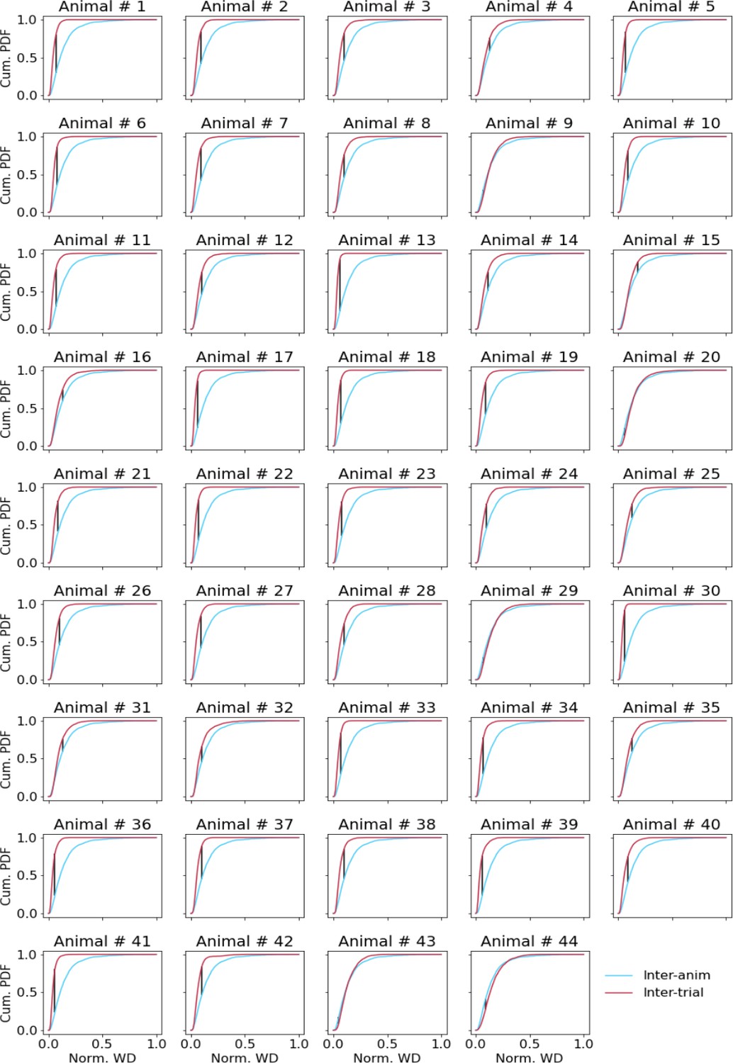
Comparing inter-trial and inter-animal pairwise Wasserstein distances (WDs).
Cumulative distributions of pairwise WDs between trial-averaged current source density (CSD) of individual animals (blue line) and pairwise WDs between single trial CSD in each animal (red lines). The black line denotes the point of maximal distance between the two distributions.
Figure 3 with 2 supplements
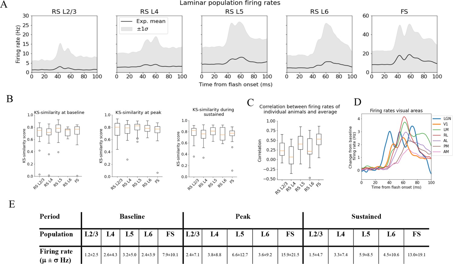
Variability in experimentally recorded spikes.
(A) Trial-averaged laminar population firing rates of regular-spiking (RS) cells, differentiated by layer, and fast-spiking (FS) cells across all layers in response to full-field flash. Black line: average across all animals. Gray shaded area: ±1 standard deviation. (B) Kolmogorov–Smirnov (KS) similarities (see ‘Materials and methods’) between the trial-averaged firing rates of each individual animal and the average firing rate over cells from all animals (black line in A) at baseline (the interval of 250 ms before flash onset), peak evoked response (from 35 to 60 ms after flash onset), and during the sustained period (from 60 to 100 ms). (C) Correlations between trial-averaged firing rates of individual mice and all mice (0–100 ms after flash onset). (D) Baseline-subtracted evoked firing rates for excitatory cells in seven visual areas (average over trials, neurons, and mice). Note the strong, stimulus-triggered gamma-range oscillations in the firing of lateral geniculate nucleus (LGN) neurons (blue). (E) Mean (μ) ± standard deviation (σ) of population firing rates during baseline, peak evoked response, and the sustained period. Averaged across trials, neurons and time windows defined above.
Figure 3—figure supplement 1

Classifying cell types in experimental data.
Distributions of waveform duration in cells from lateral geniculate nucleus (LGN), V1, and latero-medial (LM) and the threshold (red line) between classifying as regular-spiking (RS) or fast-spiking (FS).
Figure 3—figure supplement 2

Number of cells in each population in experimental data.
Left: number of regular-spiking (RS) and fast-spiking (FS) in each layer in individual animals. Right: number of FS cells across all layers in V1 in individual animals.
Figure 4 with 1 supplement
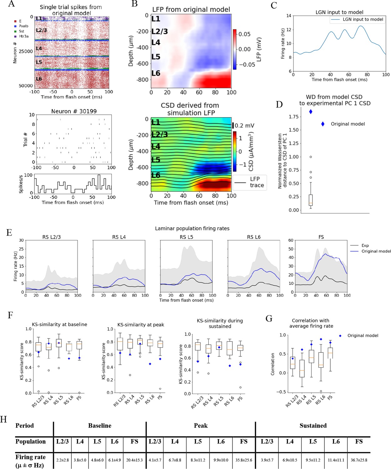
Local field potential (LFP), current source density (CSD), and spikes from simulations with the original model.
(A) Top: raster plot of all ~50,000 cells in the model’s 400 μm radius ‘core’ region spanning all layers, in a simulation of a single trial with the flash stimulus. Bottom: raster plot and histogram of spikes from 10 trials for an example cell. (B) Top: simulated LFP averaged over 10 trials of flash stimulus. Bottom: CSD calculated from the LFP via the delta iCSD method. (C) Firing rate of experimentally recorded lateral geniculate nucleus (LGN) spike trains used as input to the model. (D) Wasserstein distance between CSD from the original model (blue diamond) and PC 1 CSD from experiments together with the Wasserstein distances from experimental CSD in every animal to PC 1 CSD (boxplot), normalized to maximal distance for animals. (E) Experimentally recorded firing rates (black) and simulated firing rates (blue). (F) Kolmogorov–Smirnov (KS) similarity between firing rates in original model (blue diamond) or individual animals (boxplots) and firing rates in experiments at baseline, peak evoked response, and during the sustained period (defined in Figure 3). (G) Correlation between firing rates of model (blue diamond) or individual animals in experiments (boxplots) and average population firing rates in experiments (0–100 ms). (H) Mean (μ) ± standard deviation (σ) of model firing rates during baseline, peak evoked response, and the sustained period. Averaged across trials, neurons and time windows defined above.
Figure 4—figure supplement 1
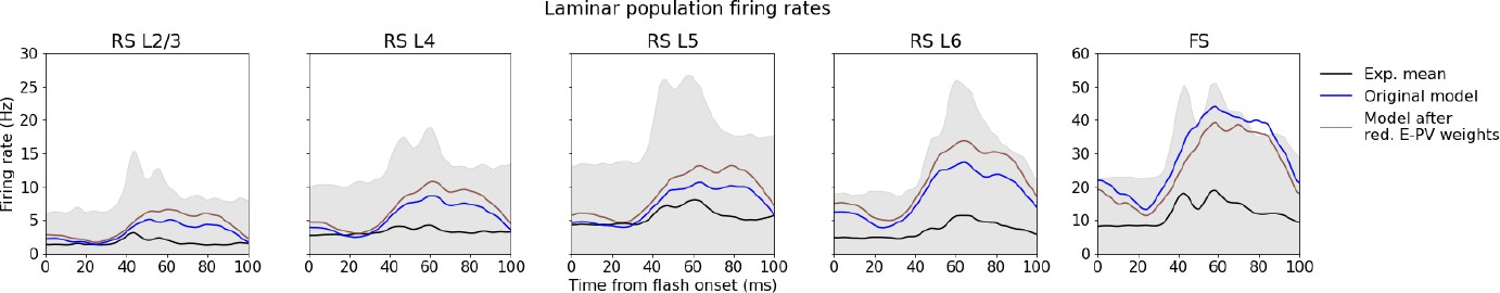
Effect of reducing recurrent inhibition.
Laminar population firing rates in the original model (blue line), in the model after reduction of recurrent excitatory synaptic weights to all Pvalb cells by 30% (brown line), and in experiments (black line).
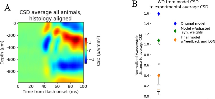
Figure 5 with 4 supplements
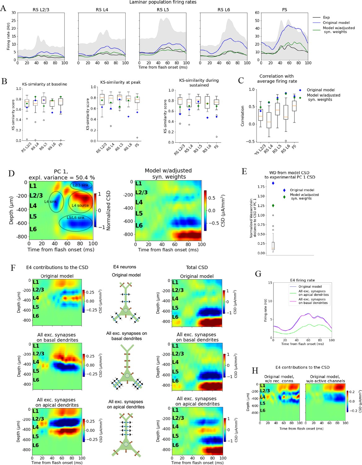
Adjusting the model to fit spikes or current source density (CSD).
(A) Average experimentally (black) and simulated firing rates of experiments in the model with adjusted recurrent synaptic weights (green) and original model (blue). Synaptic adjustments included scaling the weights from all excitatory populations to the PV cells down by 30% to reduce the firing rates in these fast-spiking populations, reducing the synaptic weights from excitatory populations to all others and increasing synaptic weights from all PV cells to all other populations to compensate for the reduced inhibition. (B) Kolmogorov–Smirnov (KS) similarity between firing rates of model versions (markers) or individual animals in experiments (boxplots) and firing rates of experiments at baseline, peak evoked response, and during the sustained (defined in Figure 3). (C) Correlation between simulated firing rates or individual animals (boxplots) and measured firing rates (0–100 ms). (D) Left: PC 1 current source density (CSD) from experiments (see Figure 2). Right: CSD resulting from simulation on model with adjusted recurrent synaptic weights. (E) Wasserstein distance between CSD from model versions and PC 1 CSD from experiments together with Wasserstein distances from CSD in animals to PC 1 CSD (boxplot). (F) Effect of different patterns of placing excitatory synapses onto layer 4 excitatory cells on this population’s contribution to the simulated CSD (left) and to the total simulated CSD (right). These synaptic placement schemes with accompanying inflowing (blue arrows) and outflowing (orange arrows) currents are illustrated in the middle. (G) Effect of synaptic placement on the simulated population firing rate. (H) Contribution of L4 excitatory cells to the simulated CSD in the model where all recurrent connections have been cut (left) and when all active channels have been removed from all cells in the model (right).
Figure 5—figure supplement 1
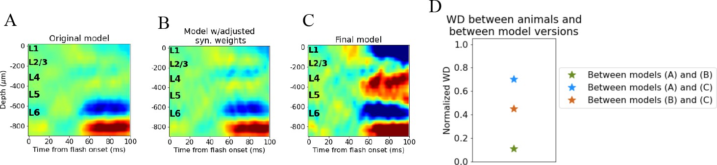
Quantifying change in simulated current source density (CSD) with adjustments to synaptic weights.
(A) CSD of original model. (B) CSD of intermediate model where synaptic weights between populations in V1 have been adjusted. (C) CSD of final model. (D) Pairwise Wasserstein distance between CSD different model versions normalized to the largest pairwise Wasserstein distance between trial-averaged CSD of individual animals. Green star: Wasserstein distance (WD) between CSD of original model (A) and intermediate model (B). Blue star: WD between CSD of original model (A) and final model (C). Orange star: WD between CSD of intermediate model (B) and final model (C).
Figure 5—figure supplement 2
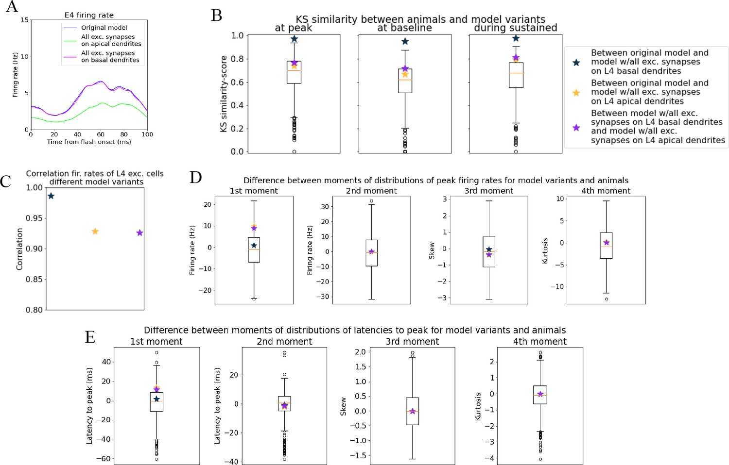
Quantifying change in spiking of L4 excitatory cells after adjusting synaptic placement.
(A) Blue line: original model where excitatory synapses onto L4 excitatory cells were placed on both basal and apical dendrites. Green line: all excitatory synapses onto L4 excitatory cells were placed only onto apical dendrites. Pink line: all excitatory synapses onto L4 excitatory cells were placed only onto basal dendrites. (B) Kolmogorov–Smirnov (KS) similarity between the model variants in (A) for average firing rates across cells in different time periods (defined in Figure 3). Boxplots represent distribution of pairwise KS similarities between animals. (C) Correlation between firing rates of model variants in (A). (D) Difference in moments of distributions of peak firing rates across cells between model variants in (A). Boxplots represent pairwise differences between animals. (E) Difference in moments of distributions of latencies to peak firing rate across cells between model variants in (A) and pairwise differences between animals (boxplots).
Figure 5—figure supplement 3

Effects of manipulating synaptic placement onto L2/3 excitatory cells on population current source density (CSD) and spiking.
(A) CSD generated by L2/3 excitatory cells in (left) the original configuration with synapses on both apical and basal dendrites, (middle) all excitatory synapses placed on apical dendrites, and (right) all excitatory synapses placed on basal dendrites. (B) Population firing rates of L2/3 excitatory cells with different synaptic placement. Blue line: original model. Green line: all excitatory synapses onto L2/3 excitatory cells were placed only onto apical dendrites. Pink line: all excitatory synapses onto L2/3 excitatory cells were placed only onto basal dendrites. (C) Kolmogorov–Smirnov (KS) similarity between the model variants in (B) for average firing rates across cells in different time periods (defined in Figure 3). Boxplots represent distribution of pairwise KS similarities between animals. (D) Correlation between firing rates of model variants in (B). (E) Difference in moments of distributions of peak firing rates across cells between model variants in (B). Boxplots represent pairwise differences in moments between animals. (F) Difference in moments of distributions of latencies to peak firing rate across cells between model variants in (B) and between animals (boxplots).
Figure 5—figure supplement 4

Effects of manipulating synaptic placement onto L5 excitatory cells on population current source density (CSD) and spiking.
(A) CSD generated by L5 excitatory cells in (left) the original configuration with synapses on both apical and basal dendrites, (middle) all excitatory synapses placed on apical dendrites, and (right) all excitatory synapses on basal dendrites. In all cases, the synapses were placed within 200 μm from the soma to have the same ranges as was used for L4 and L2/3 cells in Figure 5 and Figure 5—figure supplement 3, respectively. (B) Population firing rates of L5 excitatory cells with different synaptic placement. Blue line: original model configuration with synapses on both apical and basal dendrites, Green line: all excitatory synapses onto L5 excitatory cells were placed only onto apical dendrites. Pink line: all excitatory synapses onto L5 excitatory cells were placed only onto basal dendrites. (C) Kolmogorov–Smirnov (KS) similarity in average firing rates across cells in different time periods (defined in Figure 3) between the model variants in (B). Boxplots represent distribution of pairwise KS-similarities in animals. (D) Correlation between firing rates of model variants in (A). (E) Difference in moments of distributions of peak firing rates across cells between model variants in (B). Boxplots represent pairwise differences in moments between animals. (F) Difference in moments of distributions of latencies to peak firing rate across cells between model variants in (B) and between animals (boxplots).
Figure 6 with 9 supplements
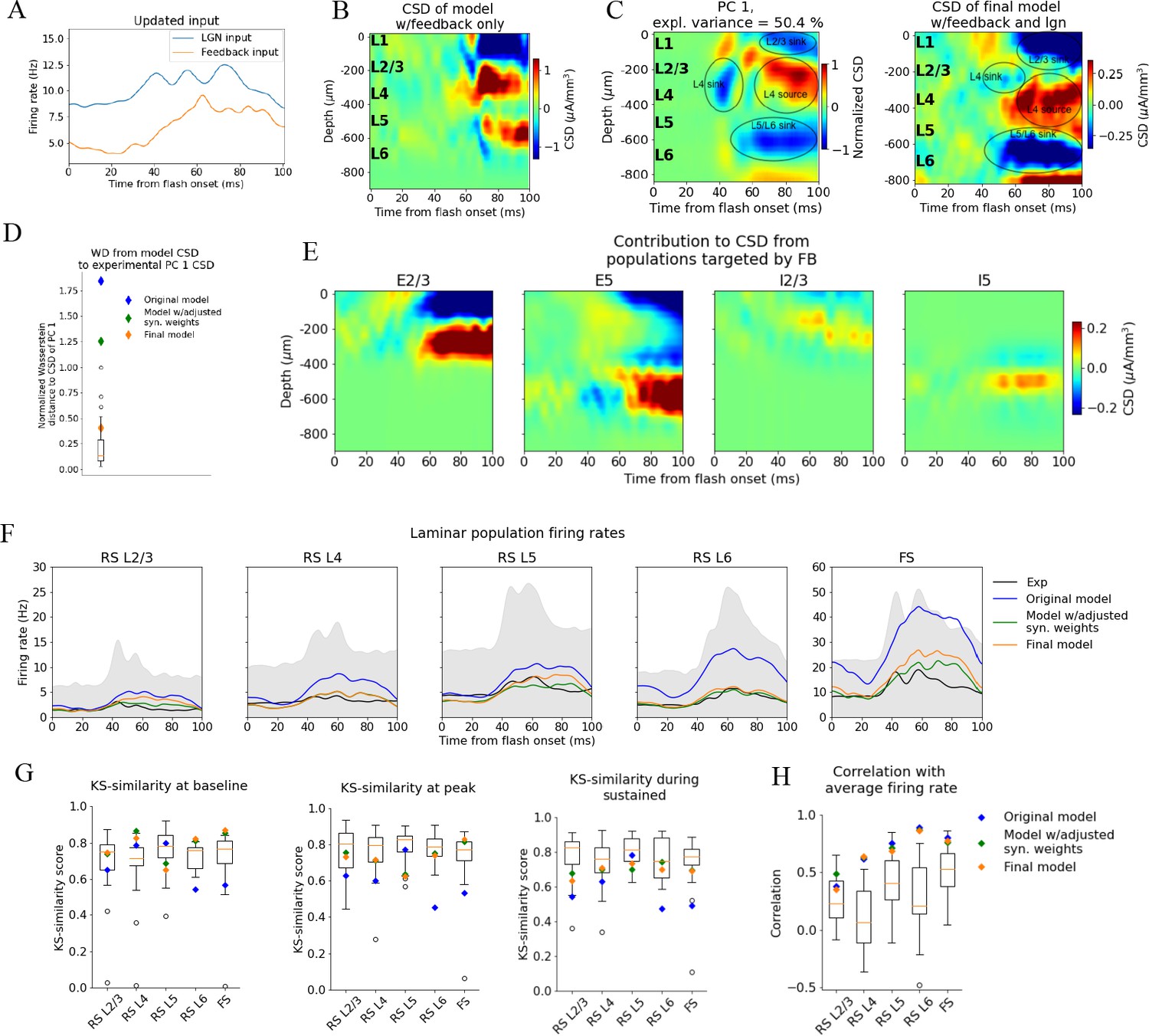
Introducing feedback from latero-medial (LM) to V1 in the model.
(A) Firing rate of the experimentally recorded lateral geniculate nucleus (LGN) and LM units used as input to the model. (B) Total current source density (CSD) resulting from simulation with input only from the LM. (C) Left: PC 1 CSD from experiments (see Figure 2). Right: total CSD from simulation with both LGN input and LM input. (D) Wasserstein distance between CSD from model versions and PC 1 CSD from experiments together with Wasserstein distances from CSD in animals to PC 1 CSD (boxplot). (E) Population contributions from populations that receive input from LM. (F) Average population firing rates of experiments (black line) and model versions. (G) Kolmogorov–Smirnov (KS) similarity between simulated firing rates or individual animals (boxplots) and recorded firing rates at baseline, peak evoked response, and the sustained period (defined in Figure 3). (H) Correlation between simulated and experimentally recorded firing rates (0–100 ms).
Figure 6—figure supplement 1

Effect of adjusting synaptic placement onto L6 excitatory cells.
Contributions to the total current source density (CSD) from L6 excitatory cells with the original placement of recurrent excitatory synapses uniformly along the whole length of their dendrites (left) and after moving all recurrent excitatory synapses within 150 μm from the soma.
Figure 6—figure supplement 2

Moments of distributions of peak firing rate in model versions and experiments for different populations.
Boxplots represent data for different animals, diamonds represent model versions. (A) First moment (mean). (B) Second moment (standard deviation). (C) Third moment (skewness). (D) Fourth moment (kurtosis).
Figure 6—figure supplement 3

Moments of distributions of latency to peak of firing rates in model versions and experiments in different populations.
Boxplots represent data for different animals, diamonds represent model versions. (A) First moment (mean). (B) Second moment (standard deviation). (C) Third moment (skewness). (D) Fourth moment (kurtosis).
Figure 6—figure supplement 4

Relative change in peak firing rates between neighboring populations.
(A) From regular-spiking (RS) cells in L2/3 to RS cells in L4. (B) From RS cells in L4 to RS cells in L5. (C) From RS cells in L5 to RS cells in L6. (D) From all RS cells in V1 to all FS cells in V1. Boxplots represent data for different animals, diamonds represent model versions.
Figure 6—figure supplement 5

Moments of distributions of greatest curvature in firing rate across cells.
Diamonds represent model versions and boxplots represent moments calculated for different animals. (A) First moment (mean). (B) Second moment (standard deviation). (C) Third moment (skew). (D) Fourth moment (kurtosis).
Figure 6—figure supplement 6

Orientation and direction selectivity in final model.
Rate at preferred direction (A), direction selectivity index (B), and orientation selectivity index (C) in layer populations of model (blue) and in experiments (gray).
Figure 6—figure supplement 7

Current source density (CSD) analysis after aligning experimental CSD plots to landmarks rather than histology.
(A) Example CSD plot with landmarks used for alignment marked (white stars). (B) Top: PC 1 CSD after application of principal component analysis (PCA) on trial-averaged CSD from all animals. Bottom: Wasserstein distances to PC 1 CSD after aligning CSD to landmarks for all animals. Diamonds denote WD from CSD of model versions and boxplots denote distances from individual animals. (C) Top: CSD average across all animals after aligning to landmarks. Bottom: Wasserstein distances to average CSD after alignment to landmarks for both model versions and animals.
Figure 6—figure supplement 8
Priincipal component analysis (PCA) on landmark aligned current source density (CSD).
(A) Left: cumulative variance explained by components. Right: variance explained by first 10 components. (B) CSD plots of the first 10 principal components explaining in total >90% of the variance in trial-averaged CSD across animals.
Figure 6—figure supplement 9
Effect of using plain average of trial-averaged current source density (CSD) from all animals instead of first principal component as target.
Wasserstein distance from model versions and individual animal CSD to plain average of trial-averaged CSD from all animals. (A) CSD averaged over trial-averaged CSD from all animals. CSD aligned to histology. (B) Wasserstein distance from CSD of model versions (diamonds) and individual animals (boxplot) to CSD averaged over all animals (normalized to largest distance from the CSD of an individual animal to the average CSD).
Figure 7 with 3 supplements
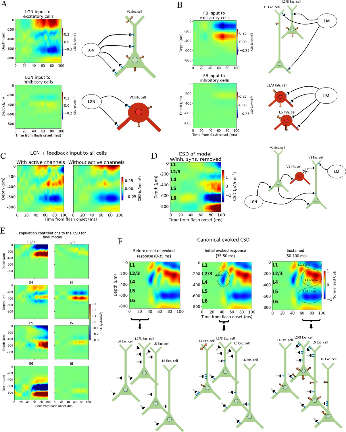
Biophysical origin of canonical current source density (CSD).
(A) Sinks and sources generated from thalamocortical and (B) feedback synapses. The schematics illustrate which synapses cause the observed sinks and sources. Blue arrows indicate inflowing current (sinks), while orange arrows indicate outflowing current (sources). (C) Total CSD from thalamocortical and feedback synapses (without recurrent connections) with (left) and without (right) active channels in the V1 neurons. (D) Total CSD of model with both thalamocortical and feedback input when inhibitory synapses are removed (cross indicates removed connection). (E) Population contributions to the total CSD in final model with both lateral geniculate nucleus (LGN) and feedback input and recurrent connections. (F) Summary of biophysical origins of the main contributions to the sinks and sources in the canonical CSD in different periods of the first 100 ms after flash onset. More arrows mean more current. Left: before onset of evoked response (0–35 ms). The average inflowing and outflowing current in V1 neurons is zero in this time window. Middle: initial evoked response (35–50 ms). The L4 sink is primarily generated by inflowing current thalamocortical synapses onto L4 excitatory cells. Right: sustained evoked response (50–100 ms). The L5/L6 sink is primarily due to inflowing currents from thalamocortical synapses and recurrent excitatory synapses. Inflowing current at synapses from higher visual areas (HVAs) onto apical tufts of L2/3 and L5 excitatory cells generates, in part, the L2/3 sink, and the resulting return current generates, in part, the L4 source in this time window.
Figure 7—figure supplement 1

Effects of removing recurrent inhibition on population current source density (CSD) and firing rates.
(A) Population contributions to the total CSD and (B) laminar population firing rates in a simulation where all inhibitory synapses have been removed.
Figure 7—figure supplement 2

Effect of cell orientation on current source density (CSD) contributions of L4 inhibitory cells.
CSD contribution of L4 inhibitory cells with original orientation (left) and scrambled orientation (right).
Figure 7—figure supplement 3

Silencing feedback from latero-medial (LM) in model during evoked response.
Current source density (CSD) of (A) PC 1 computed from experiments, (B) final model, and (C) final model with feedback turned off at 60ms. (D) Trial-averaged population firing rates in experiments (black line), final model (orange line), and final model with feedback turned off at 60ms (brown line).
Appendix 1—figure 1
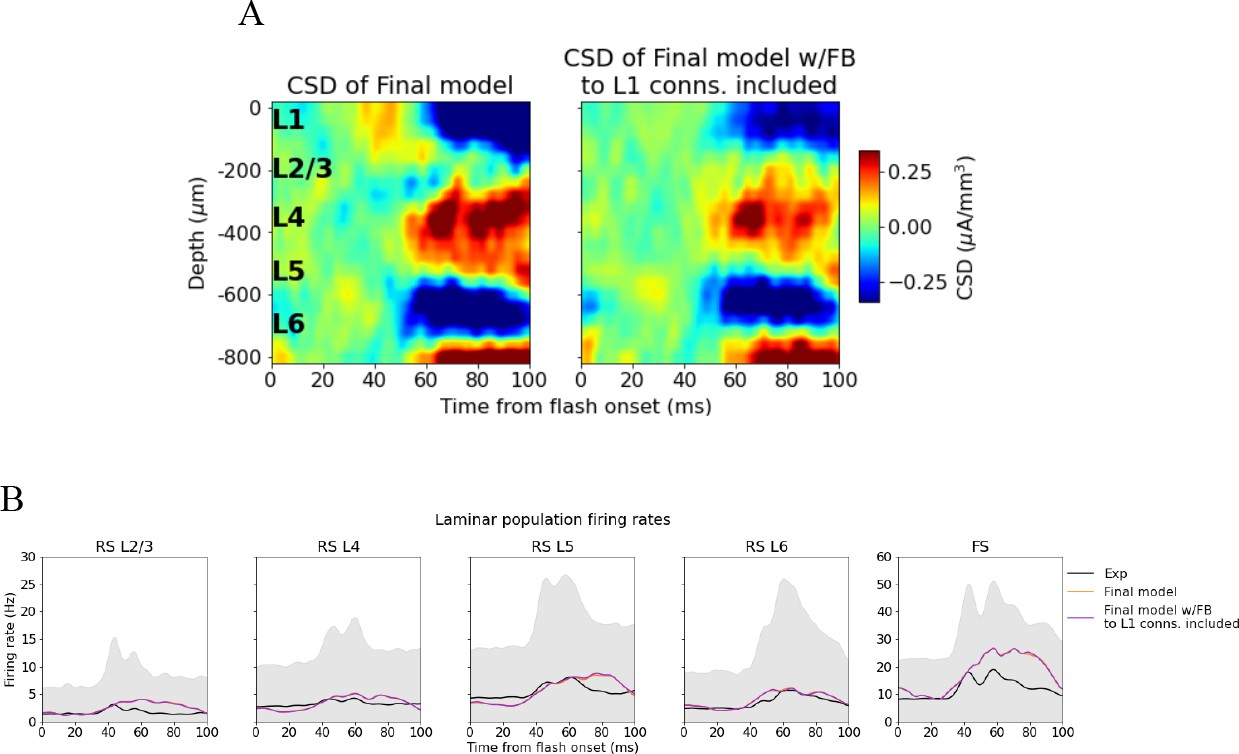
Effect of adding feedback connections from latero-medial (LM) to L1 inhibitory cells.
(A) Left: current source density (CSD) from simulation of final model version without connections from LM to L1 inhibitory cells. Right: CSD from simulation of final model version with connections from LM to L1 inhibitory cells included. (B) Population firing rates of experiments (black line), final model without connections between LM and L1 inhibitory cells (orange line), final model with connections between LM and L1 inhibitory cells included (purple colored line).
Author response image 1

ICA decomposition of experimental CSD and simulated CSD.
(A) Two examples of applying ICA on trial averaged CSD of animals. Four resulting independent components are displayed from left to right, and the trial averaged CSD of the example animal is shown in the rightmost plot. (B) Four independent components resulting from applying ICA to trial averaged CSD from the simulation on the final model version.
Additional files
Download links
A two-part list of links to download the article, or parts of the article, in various formats.
Downloads (link to download the article as PDF)
Open citations (links to open the citations from this article in various online reference manager services)
Cite this article (links to download the citations from this article in formats compatible with various reference manager tools)
Uncovering circuit mechanisms of current sinks and sources with biophysical simulations of primary visual cortex
eLife 12:e87169.
https://doi.org/10.7554/eLife.87169


