From actin waves to mechanism and back: How theory aids biological understanding
- Institute of Physics and Astronomy, University of Potsdam, Germany
- Department of Mathematics, University of British Columbia, Canada
- Department of Chemical and Biological Physics, Weizmann Institute of Science, Israel
- Swiss Institute for Dryland Environmental and Energy Research, Blaustein Institutes for Desert Research, Ben-Gurion University of the Negev, Sede Boqer Campus, Israel
- Department of Physics, Ben-Gurion University of the Negev, Israel
Figures
Figure 1
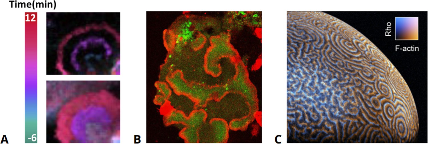
Examples of actin waves in various cell types.
(A) Human epithelial cells exhibiting actin waves (top) associated with increased levels of PIP3 (bottom). (B) Actin waves (red) enclosing areas of elevated PIP3 levels (green) in an oversized D. discoideum cell, taken from data presented in Gerhardt et al., 2014a. (C) Waves of actin and Rho in the cortex of an immature Xenopus oocyte, modified from Michaud et al., 2022.
© 2020, Elsevier. Figure 1A is reprinted from Figure 1A from Zhan et al., 2020, with permission from Elsevier. It is not covered by the CC-BY 4.0 license and further reproduction of this panel would need permission from the copyright holder.
Box 1—figure 1
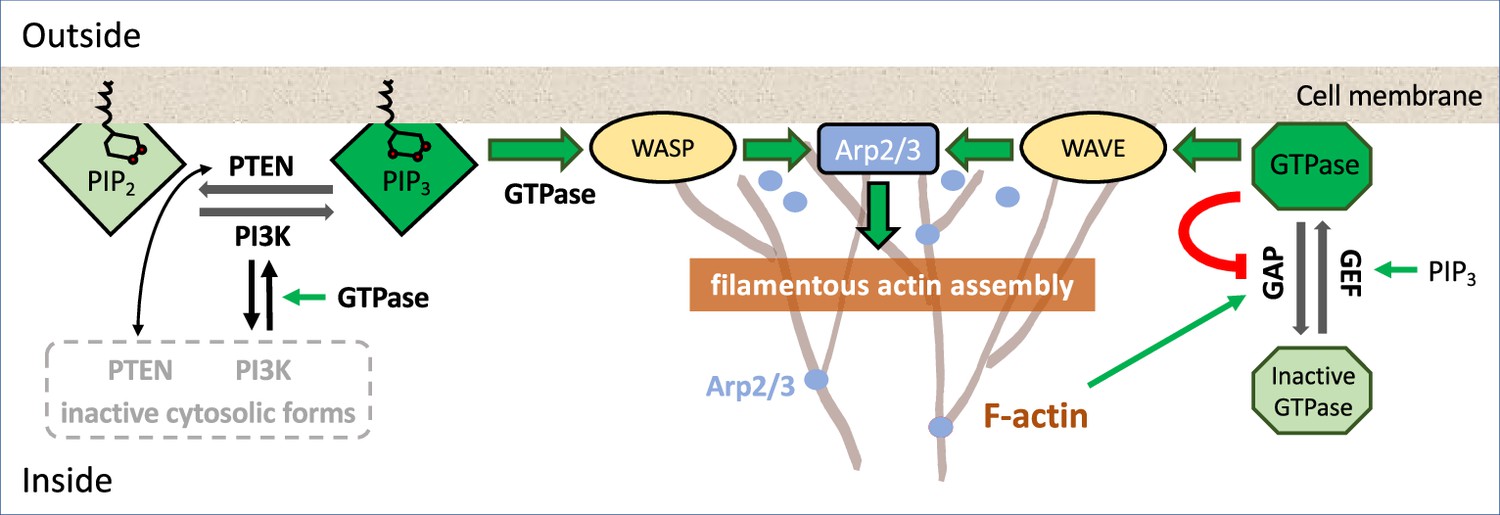
An example of signaling pathways.
Schematic diagram of a partial set of key players signaling to F-actin assembly; colored lines represent interconversion (black), positive feedback (green), negative feedback (red), and dark (light) shades of similar background/text colors denote active (inactive) forms. For more detailed biochemical pathways, see, for example, Devreotes et al., 2017; Avila Ponce de León et al., 2021.
Figure 2
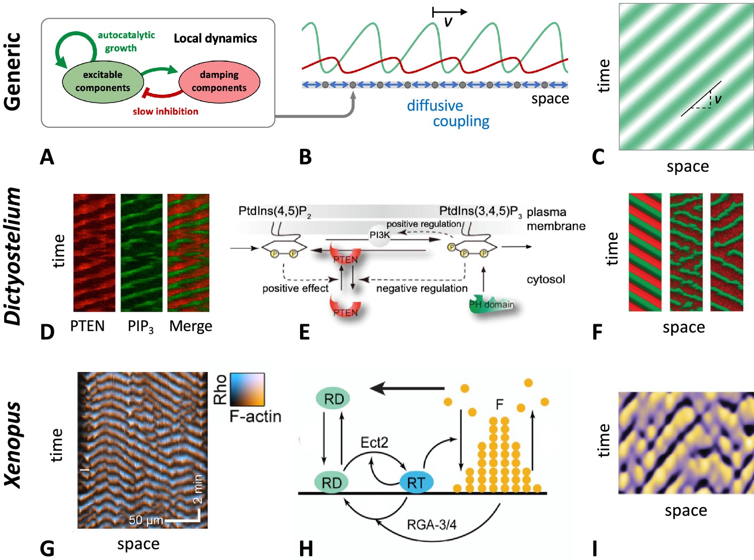
General principle of actin wave formation.
Most actin wave models are based on local nonlinear processes that involve positive and negative feedbacks between interacting species (A). In an extended system with spatial coupling, such as diffusive transport (B), this may give rise to propagating waves (C), where is the wave propagation (group) speed. Examples of actin waves and models in D. discoideum (D–F) and Xenopus oocytes (G–I) showing kymographs of the experimentally observed waves (D, G), model schematics (E, H), and simulations (F, I). The models proposed by Arai et al., 2010; Shibata et al., 2012; Shibata et al., 2013 consider active PTEN, PIP2, and PIP3, and assume conservation of PTEN. The models in Goryachev et al., 2016; Michaud et al., 2022 are based on Rho (RD, RT) and its GAP (RGA-3/4) interacting with F-actin (F). (D–F) were modified from Arai et al., 2010, Figures 1D, 5A and D, respectively. (G–I) were modified from Michaud et al., 2022, Figures 2C, 7A and E, respectively.
Figure 3
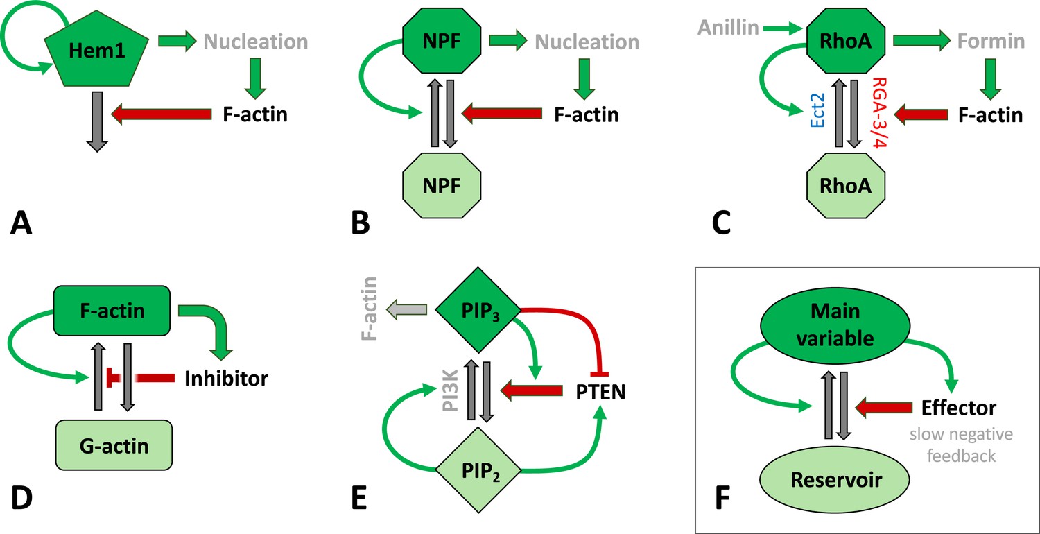
Schematic representation of signaling mechanisms for actin waves identified in various species and included in many models.
Green (red) arrows correspond to positive (negative) feedback signaling (red arrows promote inactivation in A–C, E–F or inhibit actin assembly in D). Black arrows represent interconversions, and dark (light) colors of shapes correspond to active (inactive) forms of signaling agents. (A) The Hem1 complex was identified as a central component in neutrophils as modeled in Weiner et al., 2007. (B) A generic model for actin waves based on the interactions of F-actin with a nucleation promoting factor (NPF) (Doubrovinski and Kruse, 2011; Dreher et al., 2014; Holmes et al., 2012; Mata et al., 2013). A similar filament model by Carlsson, 2010 left out the autocatalysis and failed to produce well-structured waves. (C) The assembly of F-actin by the formin mDia was investigated in embryos of C. elegans (Michaux et al., 2018), where RGA3/4 was identified as the GAP. In oocytes of Xenopus and starfish, Ect2 was found to be the GEF, and RGA3/4 is recruited by F-actin (Bement et al., 2015; Goryachev et al., 2016; Michaud et al., 2021). The circuit was modeled in Goryachev et al., 2016. (D) A model for F- and G-actin and a polymerization inhibitor was proposed by Yochelis et al., 2020; Yochelis et al., 2022. There are also similar, yet more detailed versions, that identified coronin as the inhibitor (Wasnik and Mukhopadhyay, 2014) or that incorporated cortical actin/stress fibers (Bernitt et al., 2017). (E) A slightly distinct model structure for phosphoinositides and PTEN as proposed in Shibata et al., 2012. (F) Essential structure of models (A–D): The key variable is autocatalytic and promotes an effector that exerts at least one (slow) negative feedback. The circuits have been drawn to emphasize similarities in the structures and connectivities. In (B–D), the total amount of the main agent (RhoA, GTPase, or actin) was assumed to be constant.
Figure 4
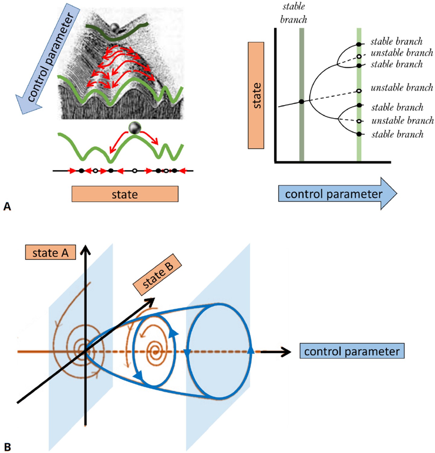
A basic description of bifurcation methodology.
(A) Phenomenological description of a bifurcation diagram using the ‘Waddington landscape.’. Left panel: The ‘state’ of a system is described by a single variable (axis labeled ‘state’). The evolution of the system with time (red arrows) is away from unstable states (open circles and mountain tops) and toward stable states (black circles and valleys). The directions of changes over time can be compressed into a flow diagram. The effect of a control parameter is shown as a shift in the geography of the hills and valleys. Right panel: A bifurcation diagram containing the information corresponding to the ‘Waddington landscape,’ where a stable state (solid line) becomes unstable (dashed line) to a pair of new stable states, a so-called ‘pitchfork’ bifurcation. The solid (dashed) lines correspond to valleys (mountain tops) in the left panel. The ‘bifurcation points’ mark parameter values, where small changes in a control parameter result in qualitative changes in the system’s behavior, e.g., when new solutions emerge at a branching point or their stability is changed. Bifurcation analysis allows us to map the ‘landscape’ of the underlying dynamical system and elucidates how various regimes of different behavior are related. In general, some branches of the bifurcation diagram may represent persistent oscillations, waves, or pulses in the system’s behavior. In (B), we schematically show a bifurcation to periodic oscillations (a.k.a. limit cycle solutions) for which the amplitude increases with distance from the bifurcation onset. Such instability is also known as a Hopf bifurcation and requires a system of at least two state variables (as opposed to a steady state pitchfork bifurcation demonstrated in (A) that may arise in models with a single variable). The shaded surfaces depict two selective phase-space projections spanned by the state variables at specific values of the control parameter, where the arrows correspond to temporal dynamics.
Box 3—figure 1
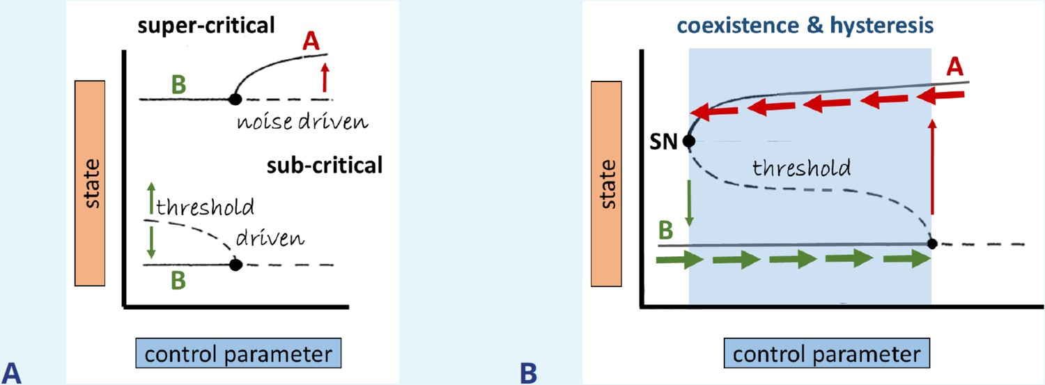
Bifurcation types, coexistence, and hysteresis.
(A) Illustration of super- vs subcritical bifurcations, where the thin red/green arrows mark the direction of the dynamics with respect to time, respectively. (B) Coexistence (bistability) is formed via the connection of branches emerging from the subcritical and saddle-node (SN) bifurcations, as indicated by the shaded region. Thick horizontal arrows indicate at which state the system persists for perturbations that do not exceed the threshold (dashed line).
Figure 5
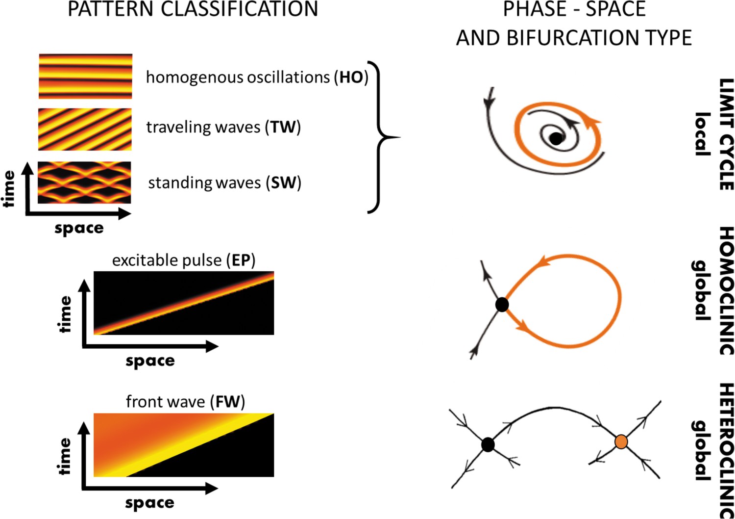
Various realizations of propagating waves and pulses.
Left panel: Three classes of propagating (time-dependent) patterns: Oscillatory waves, an excitable pulse, and a front wave (a.k.a. a traveling front); orange and black colors correspond to maximal and minimal values of the solutions, respectively. Right panel: The spatial variation of key variables across a wave (e.g., the variation in fluorescence intensity from front to back) can be represented by a trajectory in some high-dimensional ‘phase space’ spanned by the model variables (here simplified to a 2D cartoon) connecting the back state to the front state (see text), or varying periodically across the wave. Dots correspond to steady states and arrows describe flows in their vicinity. Classification of the associated local/global bifurcations through which such solutions form. Note that in phase space various oscillatory solutions all have the same geometric flow, described by a limit cycle (periodic orbit).
Box 4—figure 1
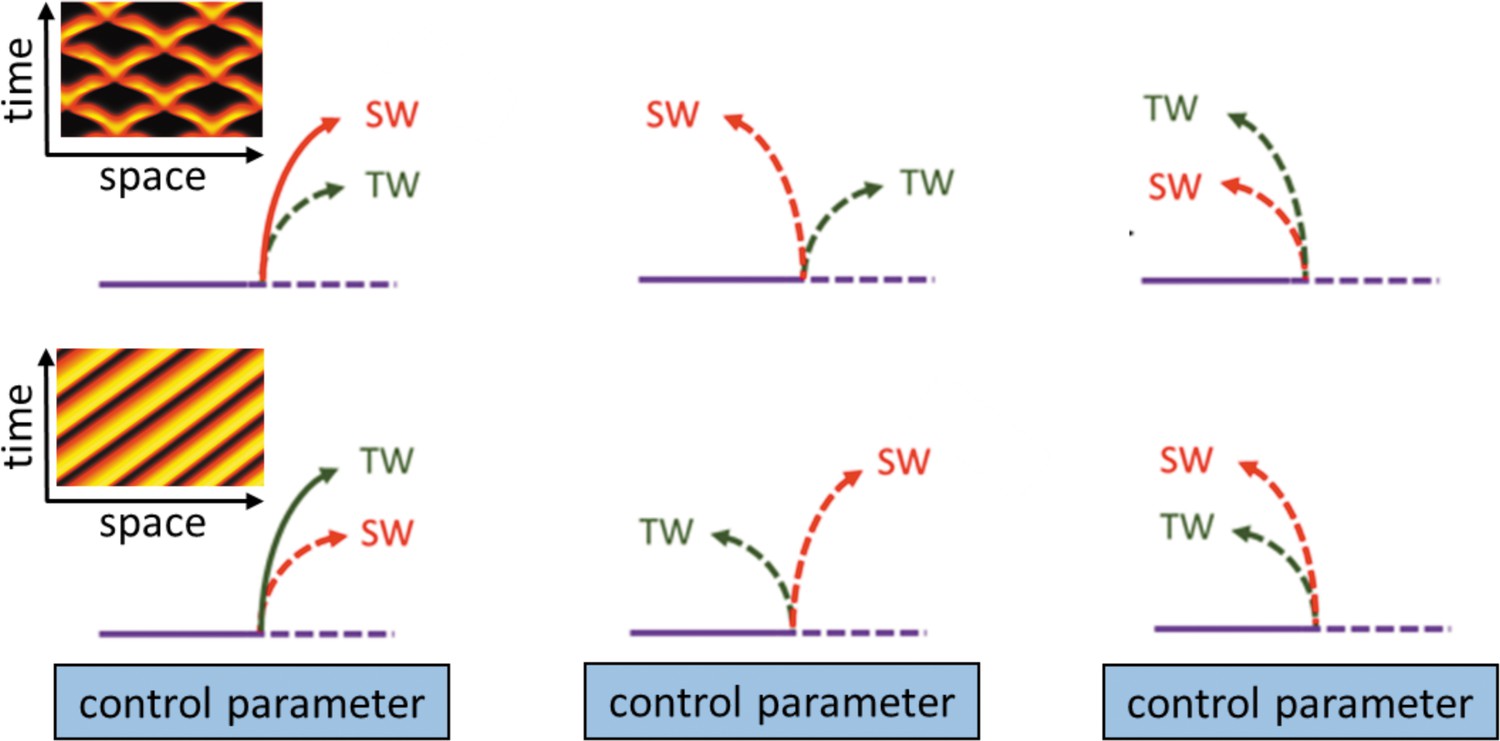
Schematic description of possible ways in which primary bifurcating traveling waves (TW) and standing waves (SW) can emerge from the finite wavenumber Hopf bifurcation.
Solid (dashed) lines indicate stable (unstable) solutions of a certain state variable (modified from Knobloch, 1986). The left insets demonstrate space-time plots of typical forms of SW employing no-flux boundary conditions (top) and TW employing periodic boundary conditions (bottom) that emerge from super-critical bifurcations.
Figure 6
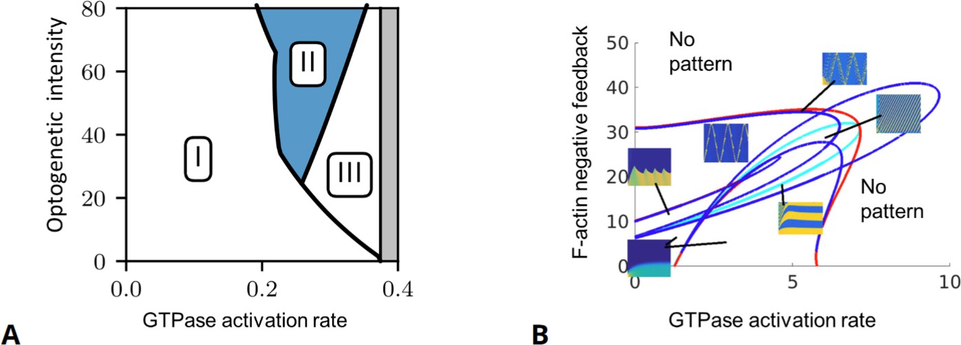
Examples of full and reduced bifurcation analyses.
(A) Full partial differential equation (PDE) bifurcation analysis of a GTPase model with no F-actin feedback. Shown are regimes of the response of a polarized model cell to a ‘polarity reversal’ stimulus. Horizontal axis: The inherent spatially uniform GTPase activation rate. Vertical axis: Optogenetic stimulus intensity that amplifies that rate in the back of the cell (% increase in GTPase activation rate for a stimulus of width 0.75 cell diameter, see experiments by O’Neill et al., 2016). The regimes represent failure to repolarize (i), reversal of polarization (ii), and loss of polarization (iii). (B) A shortcut bifurcation analysis of the actin wave model of Holmes et al., 2012 using local perturbation analysis (LPA). This two-parameter diagram displays borders of the patterning regimes (solid curves), together with typical behavior (kymographs of the full PDE solutions in one-space dimension) inside those regimes. Curves indicate Hopf (blue), fold (red) and transcritical (light blue) bifurcations in the LPA version of the model equations, as described in Liu et al., 2021. Insets: Kymographs showing spatiotemporal nucleation promoting factor (NPF) activity (yellow=high, blue=low) with time on horizontal and space on vertical axes. (A) is modified from Figure 6 in Buttenschön and Edelstein-Keshet, 2022 and (B) modified from Figure 8 in Liu et al., 2021.
© 2023, Springer Nature Switzerland. Figure 6A is reprinted from Figure 6A from Buttenschön and Edelstein-Keshet, 2022, with permission from Elsevier. It is not covered by the CC-BY 4.0 license and further reproduction of this panel would need permission from the copyright holder.
Figure 7
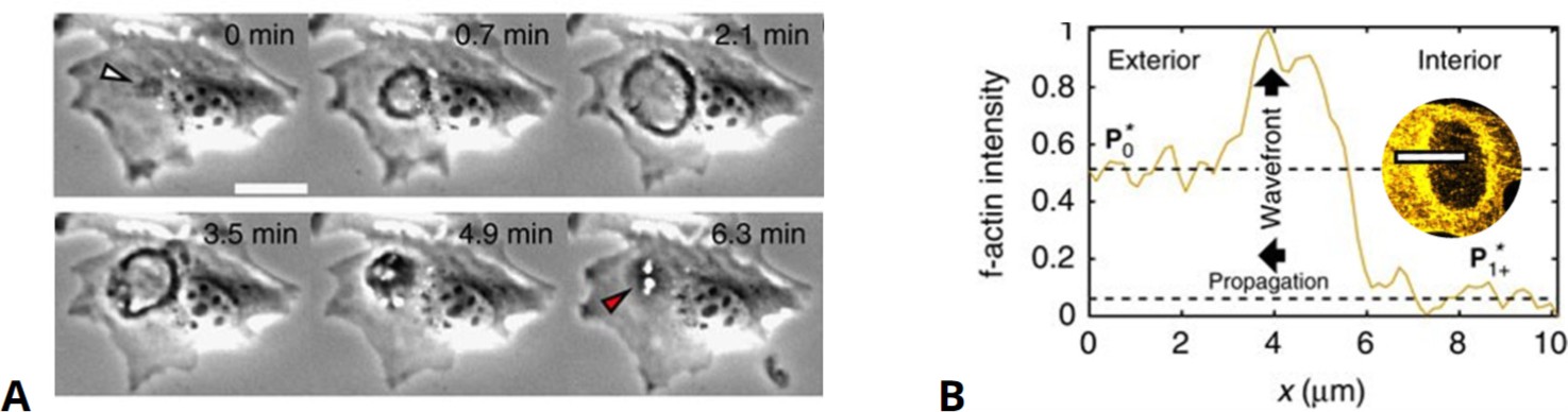
Front dynamics in circular dorsal ruffles.
(A) Experimental phase-contrast recordings of circular dorsal ruffles (CDRs) showing one cycle of the (dark colored) ring-shaped expansion and contraction. (B) F-actin concentration along the propagating wave front upon CDR expansion outward as also indicated by the top view in the inset, respectively. Modified from Bernitt et al., 2017.
Tables
Table 1
Representative mathematical models with their main variables, additional components, and methods of study.
| Species | Model | NPF | F | I | PI | Other components | Study methods | Reference |
|---|---|---|---|---|---|---|---|---|
| Dictyostelium | RD | ✔ | PIP2, PIP3, PTEN | SIM, linear BIF | Shibata et al., 2012 | |||
| Dictyostelium | RD | ✔ | ✔ | ✔ | ✔ | Arp2/3, Coronin, Rac, WASP, etc. | SIM | Khamviwath et al., 2013 |
| Dictyostelium | RD, PF | ✔ | PIP2, PIP3, PTEN, PI3K | SIM, linear BIF | Taniguchi et al., 2013 | |||
| Dictyostelium | RD | ✔ | ✔ | Monomers, Coronin | SIM | Wasnik and Mukhopadhyay, 2014 | ||
| Dictyostelium | SRD, PF | ✔ | PIP3, PTEN | SIM | Knoch et al., 2014 | |||
| Dictyostelium | RD | ✔ | Ras, PTEN, GAP, PIP3 | SIM | Fukushima et al., 2019 | |||
| Dictyostelium | SRD, LSM | ✔ | ✔ | ✔ | PIP2, Ras/Rap, PKBs, Rac, Coronin | SIM | Miao et al., 2019 | |
| Dictyostelium | SRD, PF | ✔ | ✔ | Cell edge, cytofission | SIM | Flemming et al., 2020 | ||
| Echinoderm | RD | ✔ | ✔ | Rho, Ect2 | SIM | Bement et al., 2015 | ||
| Xenopus | RD | ✔ | ✔ | Rho, Ect2 | SIM | Michaud et al., 2022; Michaud et al., 2021 | ||
| Cell extracts | RD | ✔ | ✔ | Rho, Ect2 | SIM | Landino et al., 2021 | ||
| C. elegans | ODE | ✔ | Rho, RGA3/4 | SIM | Michaux et al., 2018 | |||
| Neutrophil | ABM, ODE | ✔ | ✔ | Hem1 | SIM | Weiner et al., 2007 | ||
| Fibroblast | RD | ✔ | ✔ | Cortical actin/stress fibers, cell edge | SIM, linear BIF | Bernitt et al., 2017 | ||
| General | SRD | ✔ | ✔ | F-actin orientation | SIM | Whitelam et al., 2009 | ||
| General | ABM | ✔ | ✔ | Filament network | SIM | Carlsson, 2010 | ||
| General | RD | ✔ | ✔ | Elasticity, cell edge | SIM | Doubrovinski and Kruse, 2011 | ||
| General | RD | ✔ | ✔ | ✔ | GTPases for nucleation | SIM, LPA | Holmes et al., 2012 | |
| General | SRD, PF | ✔ | Cell edge, cell-to-cell variability | SIM | Alonso et al., 2018 | |||
| General | RD | ✔ | ✔ | G-actin | SIM, nonlinear BIF | Yochelis et al., 2022 |
-
NPF, actin nucleation promoting factor; F, F-actin; I, inhibitor; PI, phosphoinositides; SIM, simulations via numerical integration; BIF, bifurcation analysis; ABM, agent-based model; ODE, ordinary differential equations; RD, reaction-diffusion system; PF, phase field equations; SRD, stochastic-reaction-diffusion system; LPA, local perturbation analysis; LSM, level set method.
Download links
A two-part list of links to download the article, or parts of the article, in various formats.
Downloads (link to download the article as PDF)
Open citations (links to open the citations from this article in various online reference manager services)
Cite this article (links to download the citations from this article in formats compatible with various reference manager tools)
From actin waves to mechanism and back: How theory aids biological understanding
eLife 12:e87181.
https://doi.org/10.7554/eLife.87181


