A dynamical computational model of theta generation in hippocampal circuits to study theta-gamma oscillations during neurostimulation
- University of Bordeaux, CNRS, IMN, France
- University of Bordeaux, INRIA, IMN, France
- University of Bordeaux, CNRS, Bordeaux INP, France
Figures
Figure 1 with 1 supplement
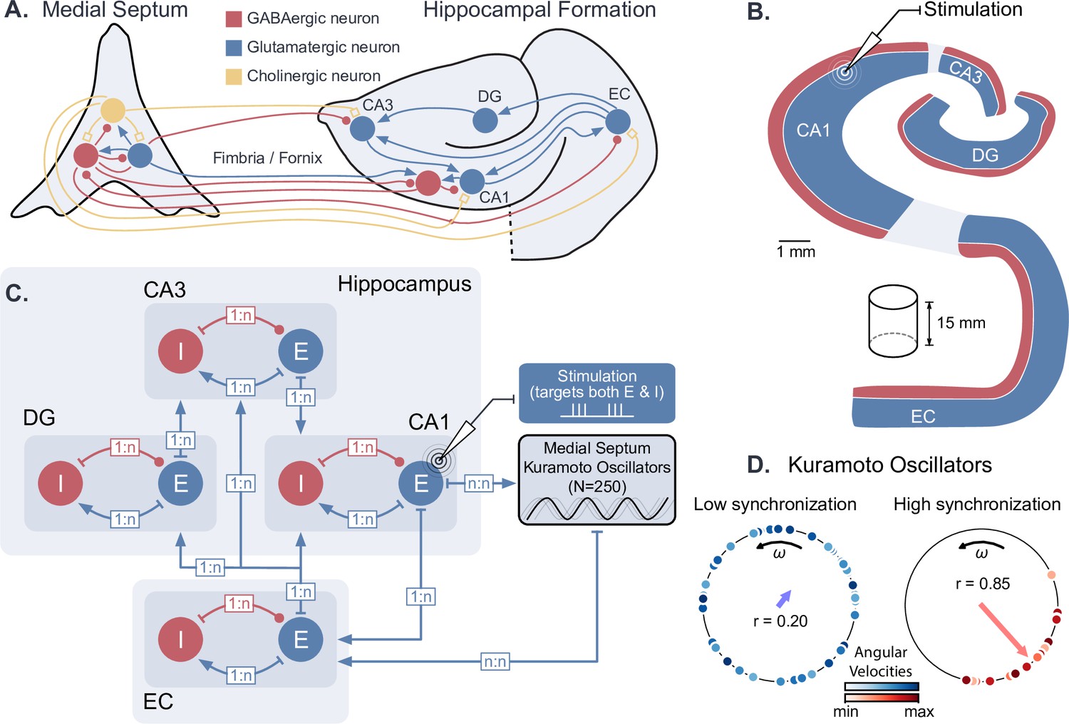
Dynamical computational model of the hippocampal formation and medial septum oscillatory drive.
(A) Anatomical representation of the neuronal types and interconnections within and between the medial septum and the hippocampal formation (EC: entorhinal cortex, DG: dentate gyrus, CA3 and CA1 fields of the hippocampus). (B) Simplified anatomy of the hippocampal formation, modeled as a 15-mm-thick cylindrical slice, with spatially segregated excitatory and inhibitory neurons (blue: excitatory neurons, consisting of granule cells in DG and pyramidal cells in other areas; red: inhibitory basket cells). (C) Model architecture and connectivity. Each area is comprised of one excitatory and one inhibitory neuronal population. Theta drive is provided through input from the medial septum, which is modeled as a set of 250 Kuramoto oscillators and receives feedback connections from CA1. Electrical stimulation Is modeled as an intracellular current affecting both excitatory and inhibitory populations in the targeted area (shown here for CA1). (D) Illustration of Kuramoto oscillators with two different levels of synchronization. Each dot represents one oscillator, its position on the circle indicates its phase and its color its angular velocity. Higher synchronization corresponds to a clustering of the dots around a similar phase. ‘’ indicates the order parameter, which is a measure of synchronization.
Figure 1—figure supplement 1
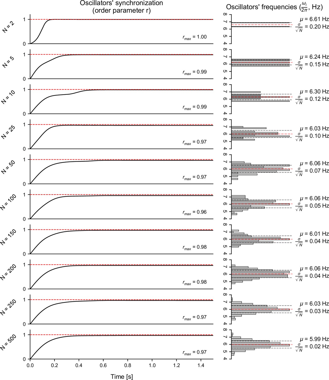
Influence of the number of Kuramoto oscillators on their collective dynamics.
Left: influence of the number of Kuramoto oscillators () on the convergence over time of the order parameter (), which is a measure of synchronization of the set of oscillators. The above results were obtained using a synchronization ratio of 25. Upon initialization, the oscillators’ natural frequencies () were normally distributed with a center frequency () of 6 Hz. Initial phases were uniformly distributed around the unit circle (). Right: histograms of the natural frequencies (), together with the distribution mean () and standard error of the mean (). As the number of oscillators increases, the mean frequency appears closer to the desired center frequency of 6 Hz, and the standard error of the mean is reduced. Overall, increasing the number of oscillators past 250 did not yield any substantial change in the convergence of the order parameter or the distribution of natural frequencies. This number of oscillators was therefore chosen for all subsequent analyses.
Figure 2 with 3 supplements
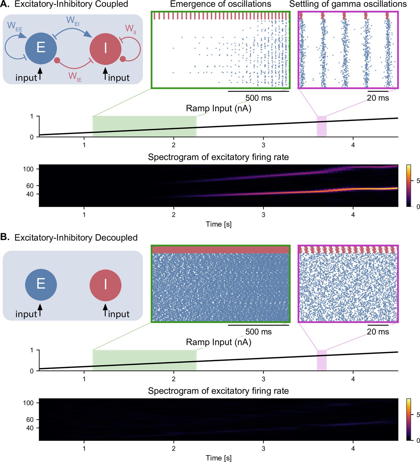
Emergence of gamma oscillations in coupled excitatory-inhibitory populations under ramping input to both populations.
(A) Two coupled populations of excitatory pyramidal neurons ( = 1000) and inhibitory interneurons ( = 100) are driven by a ramping current input (0 nA to 1 nA) for 5 s. As the input becomes stronger, oscillations start to emerge (shaded green area), driven by the interactions between excitatory and inhibitory populations. The green inset shows the raster plot (neuronal spikes across time) of the two populations during the green shaded period (red for inhibitory; blue for excitatory). When the input becomes sufficiently strong (shaded magenta area), the populations become highly synchronized and produce oscillations in the gamma range (at approximately 50 Hz). The spectrogram (bottom panel) shows the power of the instantaneous firing rate of the pyramidal population as a function of time and frequency. It reveals the presence of gamma oscillations that emerge around 2 s and increase in frequency until 4 s, when they settle at approximately 60 Hz. (B) Similar depiction as in panel A. with the pyramidal-interneuronal populations decoupled. The absence of coupling leads to the abolition of gamma oscillations, each cell spiking activity being driven by its own inputs and intrinsic properties.
Figure 2—figure supplement 1
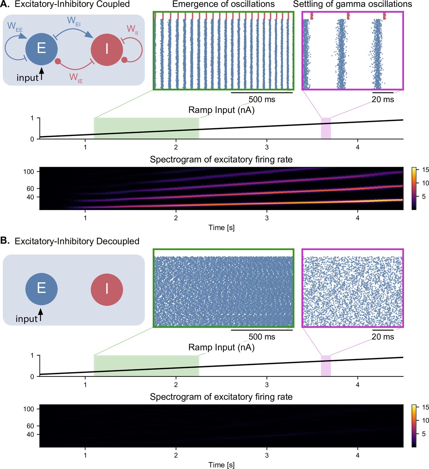
Emergence of gamma oscillations in coupled excitatory-inhibitory populations under ramping input to the excitatory population.
Similar representation as in Figure 2, but with the input provided only to the excitatory population. All conclusions remain the same. In addition, the inhibitory population does not show any spiking activity in the decoupled case.
Figure 2—figure supplement 2
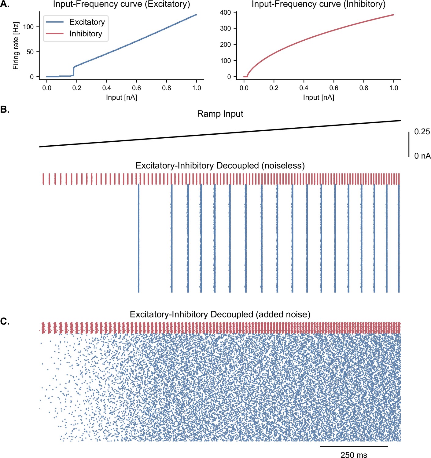
Cell-intrinsic spiking activity in decoupled excitatory and inhibitory populations under ramping input.
(A) Input-Frequency (I–F) curves for excitatory cells (left panel; pyramidal neurons with ) and inhibitory cells (right panel; interneurons, fast-spiking) used in the model. Above a certain tonic input (around 0.35 nA for excitatory and 0.1 nA for inhibitory neurons), neurons can spike in the gamma range. (B) Raster plot showing the spiking activity of excitatory (blue, = 1000) and inhibitory (red, = 100) neurons in decoupled populations under ramping input (top trace) and in the absence of noise in the membrane potential. Despite random initial conditions across neurons, oscillations emerge in both populations due to the intrinsic properties of the cells, with a frequency that is predicted by the respective I-F curves (panel A.). (C) Similar representation as panel B. but with the addition of stochastic noise in the membrane potential of each neuron. The presence of noise disrupts the emergence of oscillations in these decoupled populations.
Figure 2—figure supplement 3
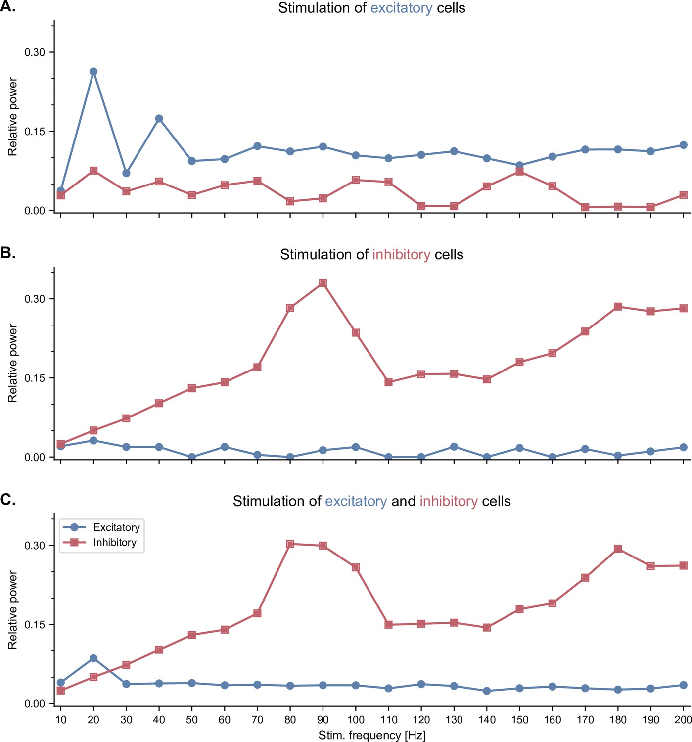
Neuronal entrainment of fast-spiking interneurons by pulsed optogenetic stimulation in the high gamma range.
All panels show the effects of pulsed optogenetic stimulation of specific cell types (A. excitatory only, B. inhibitory only, C. both excitatory and inhibitory cells) at different frequencies, similar to the experiments reported by Cardin and colleagues (Cardin et al., 2009). Pulsed stimulation was delivered continuously with a frequency ranging from 10 to 200 Hz. The relative power was calculated similarly to Cardin et al., 2009. Specifically, for each stimulation frequency, we computed first the power spectral density of the population firing rates using Welch’s method, and then the ratio between the power within a 10-Hz band centered around the stimulation frequency and the total power across all frequencies. (A) Pulsed stimulation of excitatory cells shows a higher relative power in the stimulated neurons at low frequencies (20 and 40 Hz). (B) Pulsed stimulation of inhibitory cells reveals neuronal entrainment, that is, a peak in their relative power, in the high gamma range (80-100 Hz). (C) Simultaneous pulsed stimulation of both populations reveals a strong entrainment of inhibitory cells in the high gamma range, and a more modest entrainment of excitatory cells at low frequencies.
Figure 3 with 4 supplements
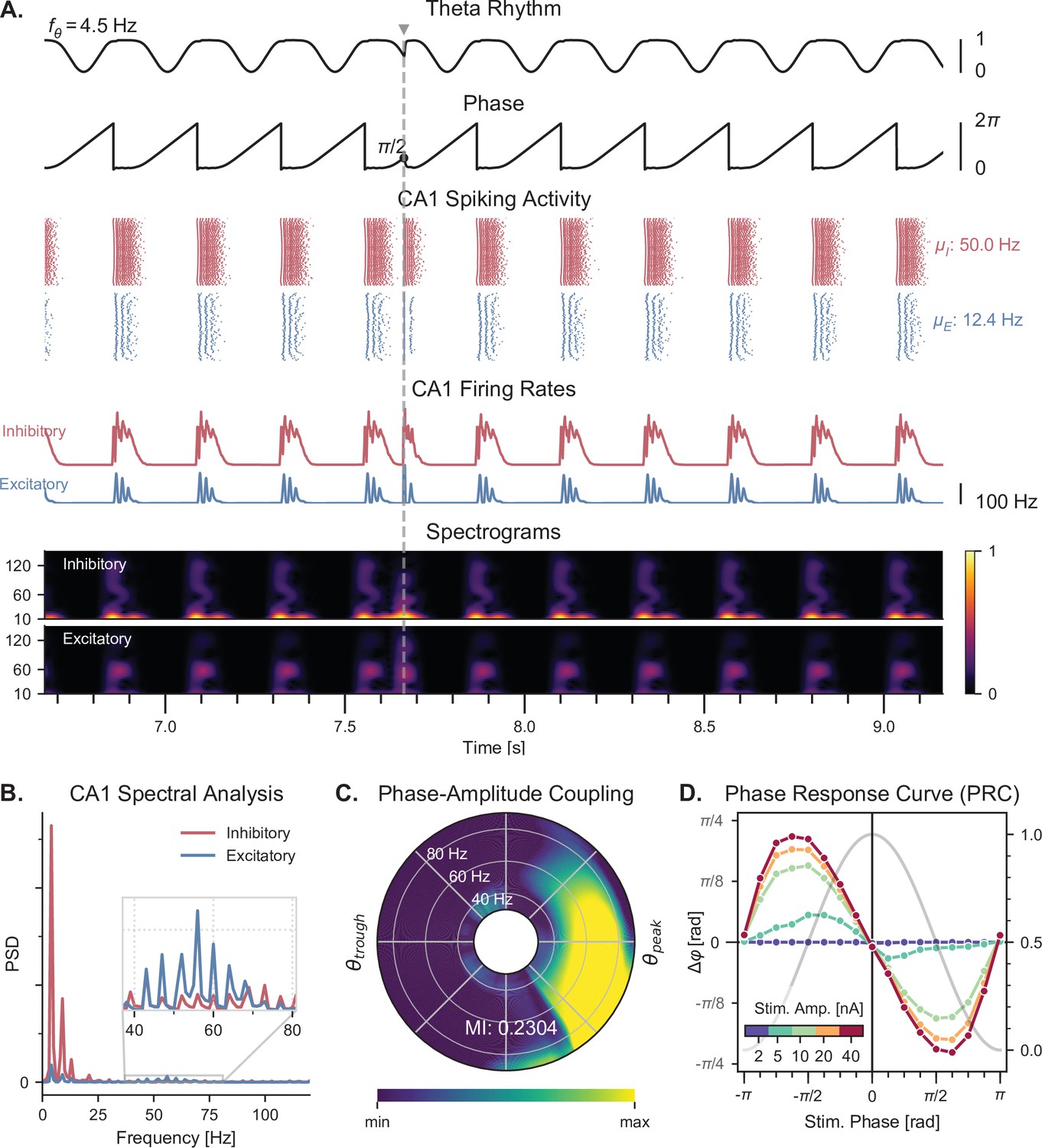
Theta-nested gamma oscillations and theta phase reset in response to a single stimulation pulse.
(A) Representative example of the network behavior, spontaneously producing theta-nested gamma oscillations and characterized by a reset of the theta phase following a single stimulation pulse (vertical grey line, applied here in CA1 at a theta phase of , that is in the middle of the descending slope). Top to bottom: theta rhythm originating from the medial septum and provided as an input to the EC (: mean oscillation frequency), instantaneous phase of the theta rhythm, raster plots indicating the spiking activity of CA1 excitatory (blue) and inhibitory (red) neurons ( and : mean firing rates within the shaded area), average population firing rates in CA1 (computed as a windowed moving average with a sliding window of 100ms with 99% overlap), spectrograms for each CA1 population (windowed short-time fast Fourier transform using a Hann sliding window: 100ms with 99% overlap). Spectrograms show gamma oscillations (around 60 Hz) modulated by the underlying theta rhythm (∼4 Hz), indicating theta-gamma PAC. Theta phase reset after stimulation is associated with a rebound of spiking activity and theta-nested gamma oscillations. (B) Power spectral densities of the CA1 firing rates. Theta peaks are found at 4 Hz for excitatory and inhibitory cells. Gamma activity is located between 40 and 80 Hz. (C) PAC as a function of theta phase and gamma frequency. The polar plot represents the amplitude of gamma oscillations (averaged across all theta cycles, see Materials and methods) at each phase of theta (theta range: 3–9 Hz, phase indicated as angular coordinate) and for different gamma frequencies (radial coordinate, binned in 10 Hz ranges), indicating that gamma oscillations between 40 and 80 Hz occur preferentially around the peak of theta. The MI gives an overall quantification of how the phase of low-frequency oscillations (3–9 Hz) modulates the amplitude of higher-frequency oscillations (40–80 Hz) (see Materials and methods and Figure 3—figure supplement 2). (D) PRC in response to a single stimulation pulse applied in CA1 at various phases of the ongoing theta rhythm and for various stimulation amplitudes (color-coded). The phase difference (left y-axis) shows the theta phase induced by the stimulation pulse (computed 2.5ms after the pulse), compared to the phase computed at the same time in a scenario without stimulation. Positive and negative phase differences indicate phase advances and delays, respectively. The grey trace shows the normalized amplitude of theta (right axis) for different phases, used to indicate the peak and trough of the rhythm. Stimulation applied in the ascending slope of theta () produced a phase advance and accelerated the rhythm towards its peak (0 radians). Conversely, stimulation during the descending slope () produced a phase delay that slowed down the rhythm. Higher stimulation amplitudes yielded a stronger effect.
Figure 3—figure supplement 1
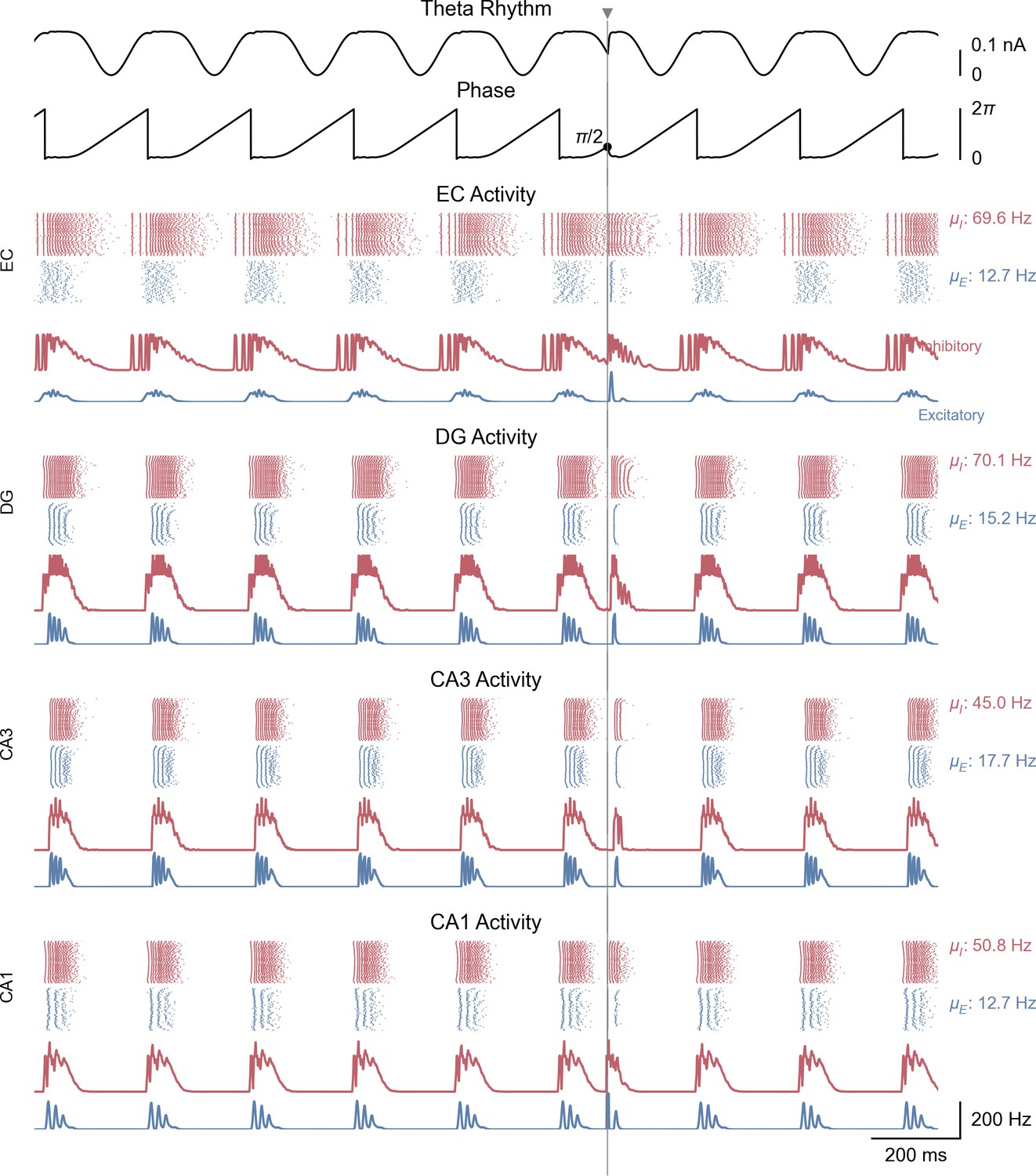
Whole-network behavior producing theta-nested gamma oscillations and theta phase reset in response to a single stimulation pulse.
This figure shows the behavior of all areas of the hippocampal formation during the simulation illustrated in Figure 3A. All areas display bursts of gamma activity that occur almost synchronously at the peak of each theta cycle in both excitatory and inhibitory neuronal populations ( and: mean firing rates within the shaded area). The CA1 excitatory population firing rate is supplied back to the medial septum. A single stimulation pulse (vertical line and grey triangle) delivered to both CA1 populations at a phase of (i.e. halfway through the descending slope) resets the phase of the theta rhythm according to the PRC shown in Figure 3D.
Figure 3—figure supplement 2
Quantification of PAC with and without noise.
(A) Quantifying PAC in the absence of noise produced inaccurate identification of the coupled frequency bands, due to the complete absence of oscillations at some frequencies. All analyses are based on the CA1 firing rates (top traces) during a representative simulation. Power spectral densities of these firing rates (left) indicate that some frequencies have a power of 0. PAC of the excitatory population was assessed using two graphical representations, the polar plot (middle) and comodulogram (right), and quantified using the MI. The comodulogram was calculated by computing the MI across 80% overlapping 1-Hz frequency bands in the theta range and across 90% overlapping 10 Hz frequency bands in the gamma range and subsequently plotted as a heat map. In the absence of noise, a slow theta frequency centered around 5 Hz is found to modulate a broad range of gamma frequencies between 40 and 100 Hz. The value indicated on the comodulogram indicates the average MI in the 3-9 Hz theta range and 40-80 Hz gamma range. As in Figure 3, the polar plot represents the amplitude of gamma oscillations (averaged across all theta cycles) at each phase of theta (theta range: 3–9 Hz, phase indicated as angular coordinate) and for different gamma frequencies (radial coordinate, binned in 1 Hz ranges). (B) Adding uniform noise to the firing rate (with an amplitude ranging between 15 and 25% of the maximum firing rate) improved the identification of the coupled frequency bands. In this case, the slower theta frequency centered around 5 Hz modulates a gamma band located between 45 and 75 Hz.
Figure 3—figure supplement 3
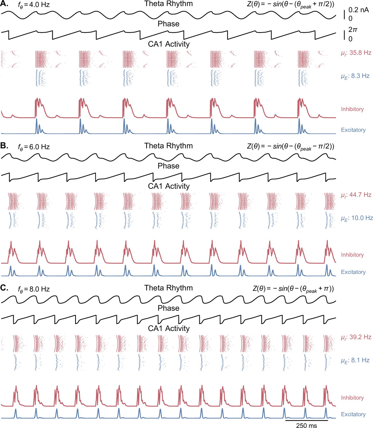
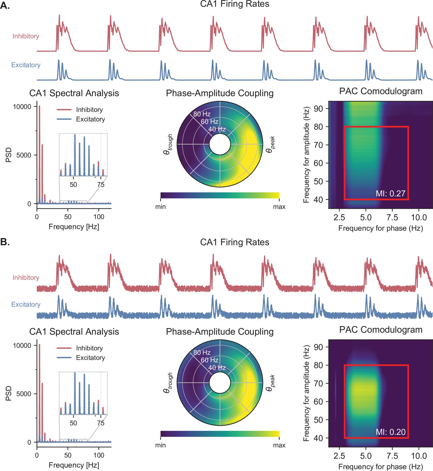
Network behavior generated by Kuramoto oscillators with non-physiological phase response functions.
Each panel is similar to Figure 3A, but with a different offset added to the phase response function of the Kuramoto oscillators (see methods, Equation 4). The center frequency was set to 6 Hz in all of these simulations. Overall, theta oscillations in these cases are less sinusoidal and show more abrupt phase changes than in the physiological case. (A) A phase offset of leads to an overall theta oscillation of 4 Hz, with a second peak following the main theta peak. (B). A phase offset of reduces the peak of theta, resetting the rhythm to the middle of the ascending phase. (C) A phase offset of or leads to the CA1 output resetting the theta rhythm to the trough of theta.
Figure 3—figure supplement 4
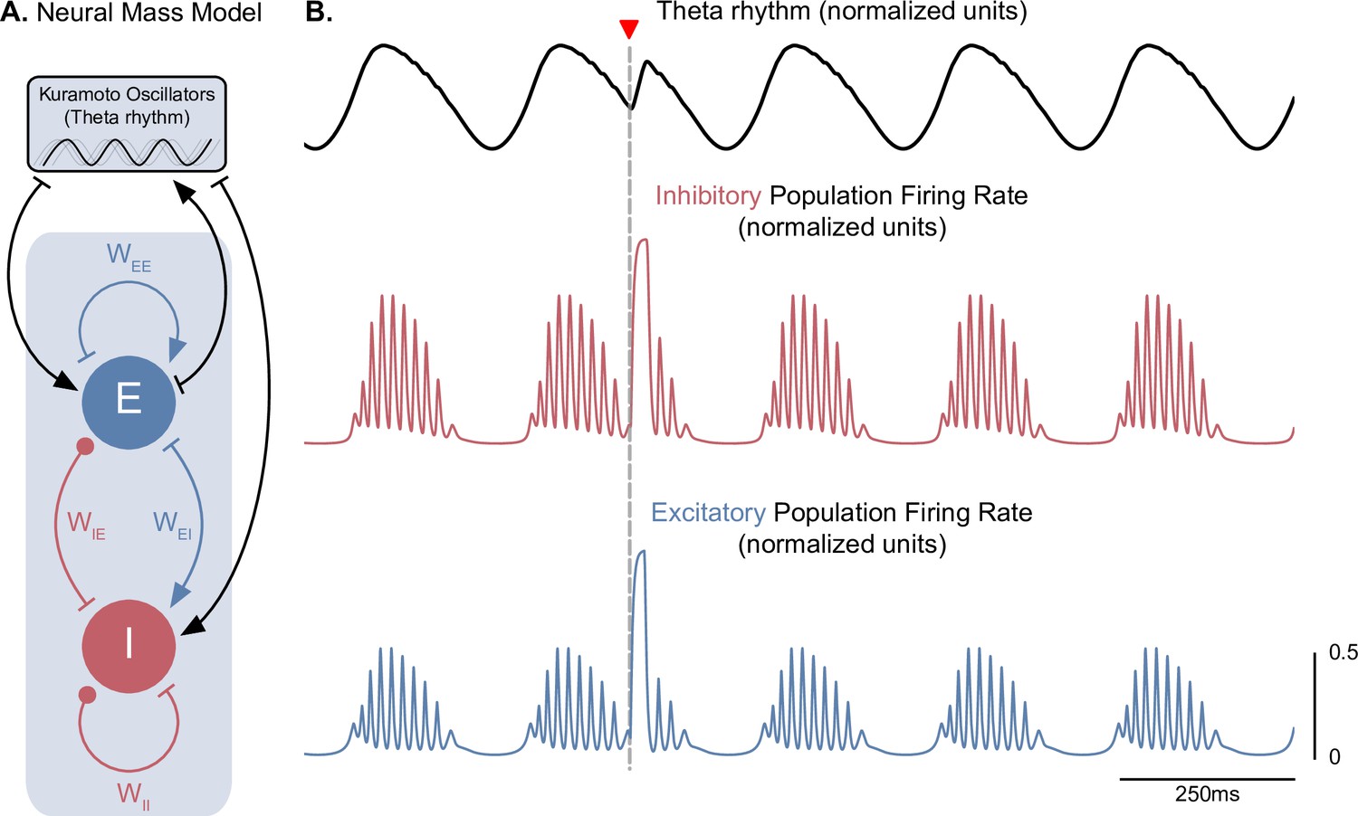
A neural mass model of coupled excitatory and inhibitory neurons driven by Kuramoto oscillators generates theta-nested gamma oscillations and theta phase reset.
(A) Two coupled neural masses (one excitatory and one inhibitory) driven by Kuramoto oscillators, which represent a dynamical oscillatory drive in the theta range, were used to implement a neural mass equivalent to our conductance-based model represented in Figure 1. Neural masses were modeled using the Wilson-Cowan formalism, with parameters adapted from Onslow et al., 2014 ( = 4.8, = = 4, = 0). (B) The normalized population firing rates exhibit theta-nested gamma oscillations (middle and bottom panels) in response to the dynamic theta rhythm (top panel). A stimulation pulse delivered at the descending phase of the rhythm to both populations (marked by the inverted red triangle) produces a robust theta phase reset, similarly to Figure 3A.
Figure 4
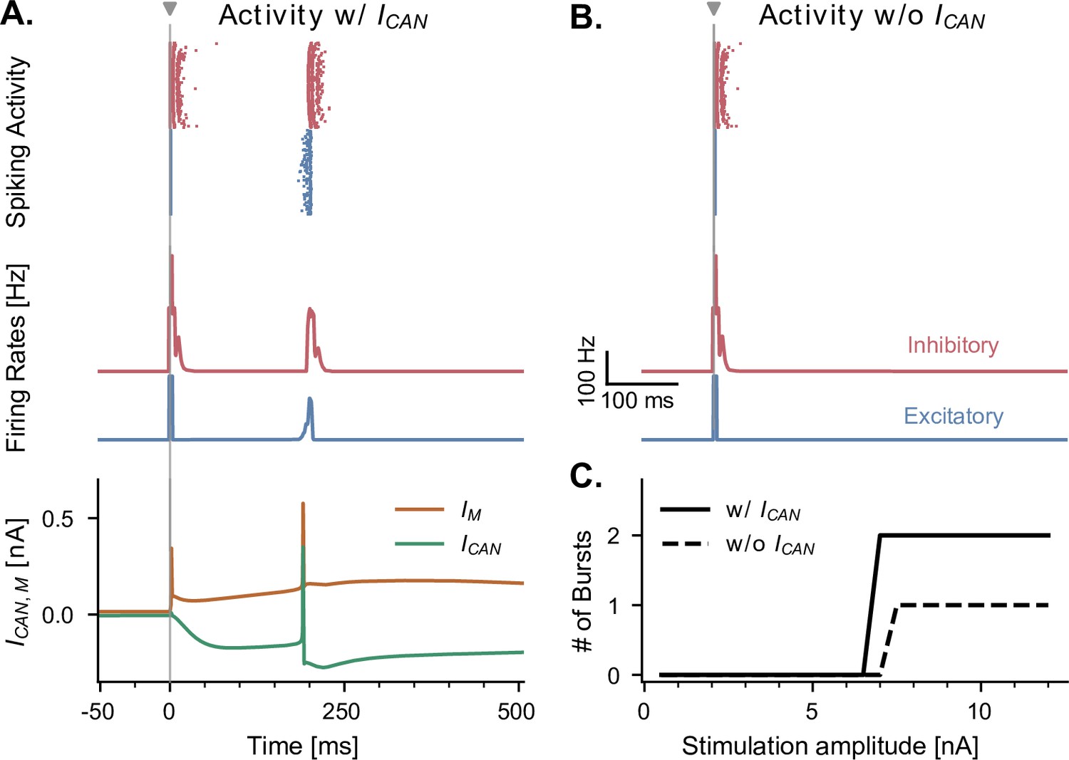
CAN and adaptation (M) currents modulate neuronal responses to single-pulse stimulation in the absence of theta input.
(A) Network response to single-pulse stimulation in the absence of medial septum input. Stimulation (grey vertical line, 10 nA, applied in CA1) induced an instantaneous burst of activity lasting about 20ms in both excitatory and inhibitory CA1 neurons, followed by a secondary burst approximately 200 ms later (raster plot and firing rate traces), associated with specific CAN- and M- currents dynamics (bottom traces, illustrated for a representative CA1 excitatory neuron). Positive () and negative () currents indicate respectively a hyperpolarizing and depolarizing effect on the cell membrane potential. (B) Similar representation as in A., but in the absence of CAN channel. Stimulation induced only a single burst of activity, indicating that CAN channels are necessary to observe a rebound of activity. (C) Number of bursts in CA1 spiking activity following a single stimulation pulse at various amplitudes (x-axis), shown both in the presence and absence of CAN channels in excitatory neurons. The absence of the CAN current leads to the abolition of the second burst, irrespective of stimulation amplitude.
Figure 5 with 5 supplements
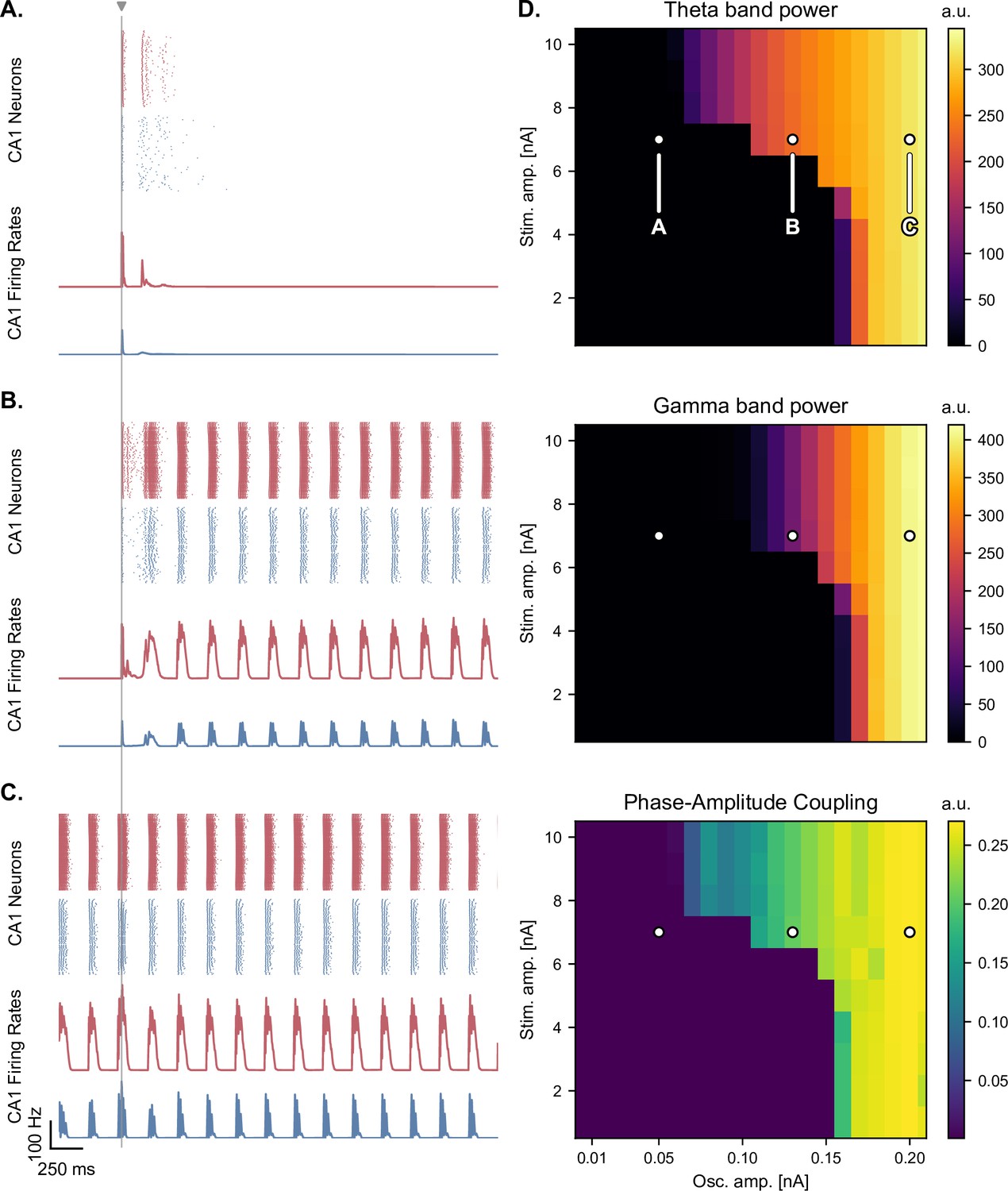
Medial septum oscillatory drive and stimulation amplitude govern the steady-state response to single-pulse stimulation.
(A-C) Network responses to single-pulse stimulation (vertical line) under medial septum input (with phase reset), shown for different amplitudes of the medial septum oscillatory drive (A-C: increasing oscillator amplitudes). (A) Low oscillatory input: stimulation induces only two bursts of spiking activity as in Figure 4. (B) Medium oscillatory input: a single stimulation pulse switches network behavior from no activity to sustained oscillations driven by the medial septum. (C) Higher oscillatory input: theta drive is capable of inducing self-sustained theta-nested gamma oscillations. In this case, stimulation is delivered at the peak of theta oscillations and does not show a pronounced effect on theta-gamma oscillations. (D) Steady-state response to single-pulse stimulation as a function of medial septum oscillatory input (x-axis) and stimulation amplitude (y-axis), characterized by three metrics: theta power (3–9 Hz), gamma power (40–80 Hz), and PAC (quantified using the MI). White dots: parameter combinations corresponding to panels A-C.
Figure 5—figure supplement 1
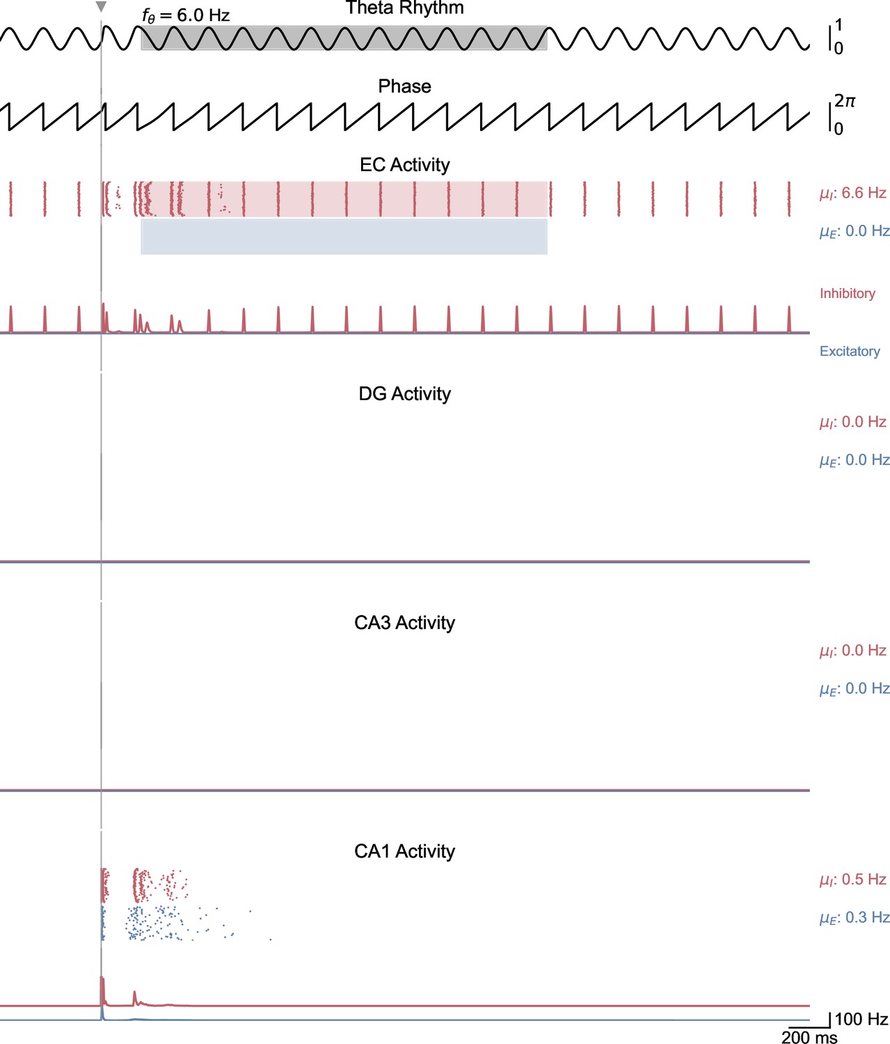
Whole-network behavior in response to single-pulse stimulation under low theta oscillatory drive.
This figure shows the behavior of all areas of the hippocampal formation during the simulation illustrated in Figure 5A. A single stimulation pulse delivered to both CA1 populations induces two bursts of spiking activity that propagate only from CA1 to EC.
Figure 5—figure supplement 2
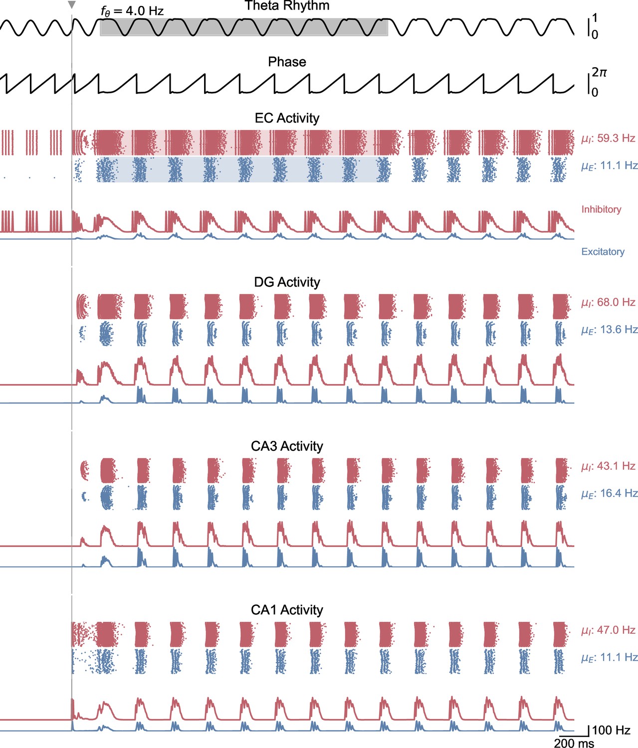
Whole-network behavior in response to single-pulse stimulation under medium theta oscillatory drive.
This figure shows the behavior of all areas of the hippocampal formation during the simulation illustrated in Figure 5B. A single stimulation pulse switches network behavior from no activity to sustained oscillations driven by the medial septum.
Figure 5—figure supplement 3
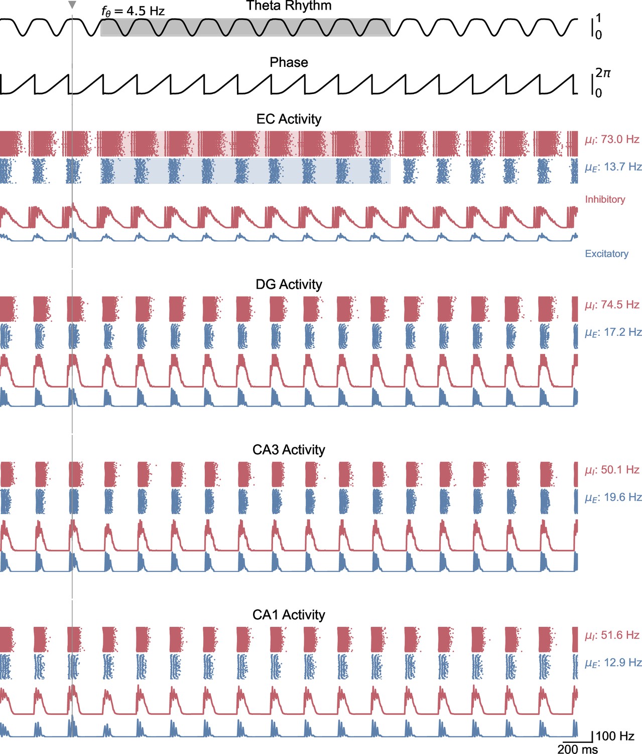
Whole-network behavior in response to single-pulse stimulation under higher theta oscillatory drive.
This figure shows the behavior of all areas of the hippocampal formation during the simulation illustrated in Figure 5C. Theta oscillatory drive is enough to induce self-sustained theta-nested gamma oscillations. In this case, stimulation is delivered at the peak of theta and does not induce a pronounced effect on theta-gamma oscillations.
Figure 5—figure supplement 4
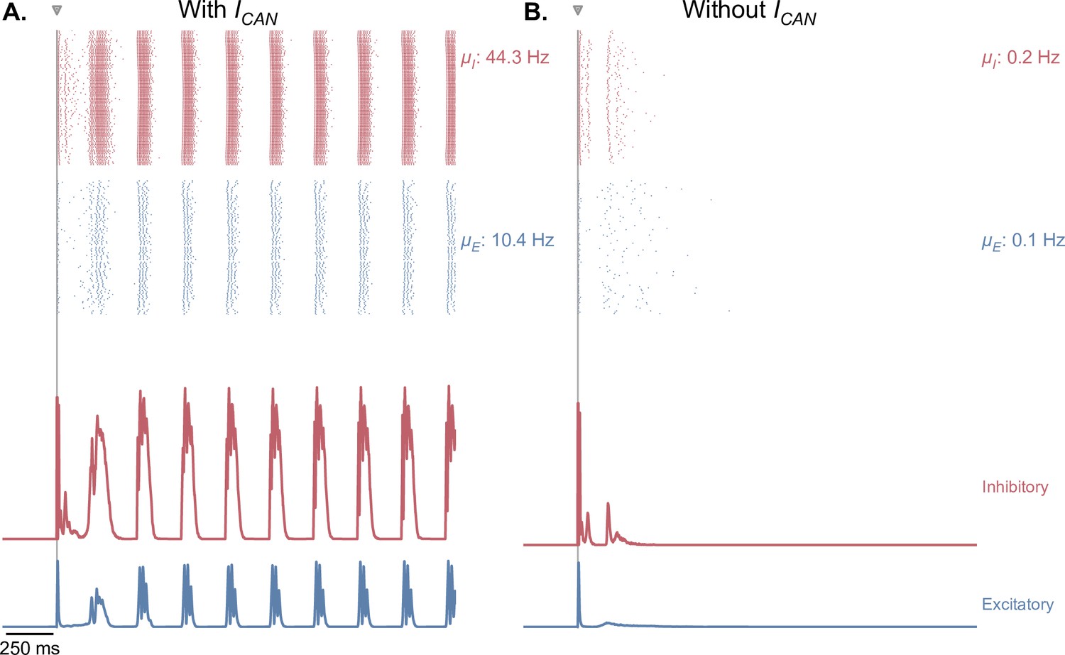
CAN currents are necessary for the production of self-sustained theta-gamma oscillations in response to single-pulse stimulation.
(A) Same as Figure 5B. (B) Similar simulation as panel A., but without the presence of CAN currents in the EC, CA3, and CA1 fields of the hippocampus. Removing CAN currents from the model abolishes self-sustained theta-nested gamma oscillations in response to a single stimulation pulse (for the parameters represented in Figure 5, point B).
Figure 5—figure supplement 5
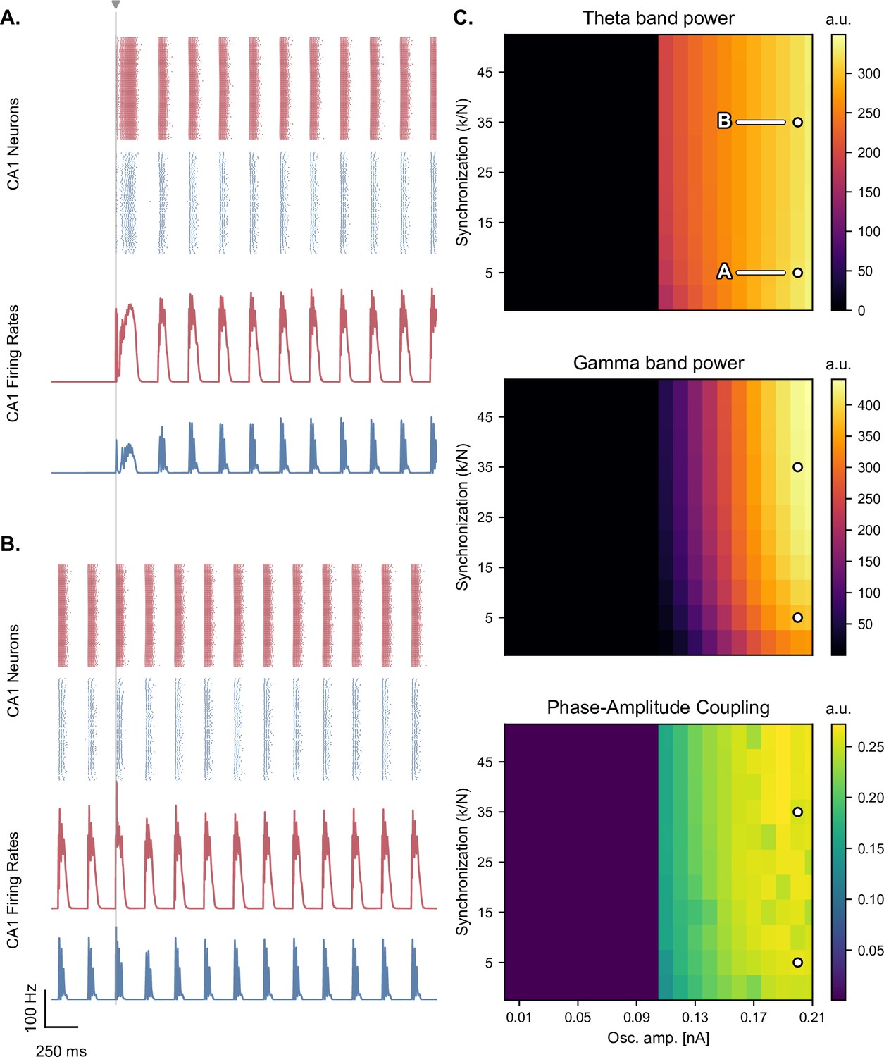
Synchronization level of the oscillators minimally affects the production of theta-nested gamma oscillations.
(A, B) Network responses to single-pulse stimulation (vertical line) under medial septum input (with phase reset), shown for different synchronization parameter ratios of the Kuramoto oscillators (A,B: of 5 and 35 respectively; stimulation amplitude: 7.0 nA). Panel B. indicates that the model can produce oscillations without external stimulation when the synchronization level is higher. (C) Steady-state response to single-pulse stimulation as a function of medial septum oscillatory input (x-axis) and synchronization parameter ratio (, y-axis), characterized by three metrics: theta power (3–9 Hz), gamma power (40–80 Hz), and PAC (quantified using the MI). White dots: parameter combinations corresponding to panels A and B.
Figure 6
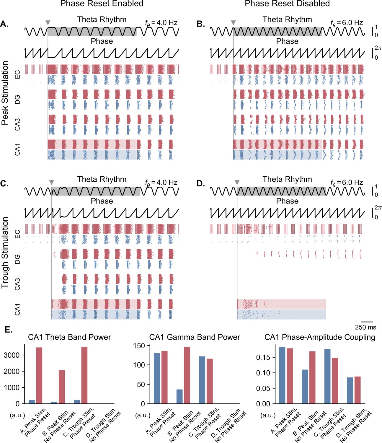
Single-pulse stimulation phase differentially affects network responses depending on the presence of theta phase reset.
All results shown here were obtained for parameters from Figure 5B (theta oscillation amplitude: 0.13 nA, stimulation amplitude: 7.0 nA). A single stimulation pulse was delivered at the peak (A, B) or trough (C, D) of the underlying theta rhythm, either in the presence (A, C) or absence (B, D) of theta phase reset. With phase reset, both peak and trough stimulation switch network behavior from no activity to sustained oscillations. Without phase reset, only peak stimulation can induce sustained oscillations. (E). Quantification of theta power, gamma power, and PAC (measured using the MI) in CA1 excitatory (blue) and inhibitory (red) populations in all four cases (metrics are computed in the shaded areas of panels A-D).
Figure 7
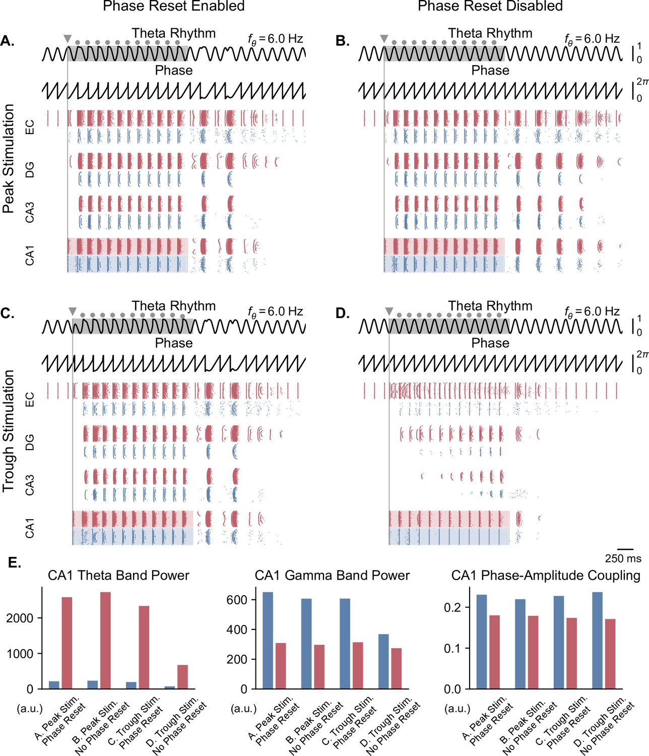
Pulse train stimulation restores theta-nested gamma oscillations depending on stimulation timing and theta phase reset.
All results shown here were obtained for parameters from Figure 5A (theta oscillation amplitude: 0.05 nA; stimulation amplitude: 7.0 nA). Representations are similar to Figure 6, with the difference that stimulation consisted of a pulse train delivered at 6 Hz for a duration of 2 s (individual pulses indicated by grey dots, first pulse by a triangle). The pulse train was delivered at the peak (A, B) or trough (C, D) of the underlying theta rhythm, either in the presence (A, C) or absence (B, D) of theta phase reset. With phase reset, both peak and trough stimulation switch network behavior from no activity to sustained oscillations. Without phase reset, only peak stimulation can induce sustained oscillations. E. Quantification of theta power, gamma power, and PAC (measured using the MI) in CA1 excitatory (blue) and inhibitory (red) populations in all four cases (metrics are computed during the pulse train, within the shaded areas of panels A-D).
Author response image 1

Figure 2.
Emergence of gamma oscillations in coupled excitatory-inhibitory populations under ramping input to both populations. (A) Two coupled populations of excitatory pyramidal neurons (NE = 1000) and inhibitory interneurons (NI = 100) are driven by a ramping current input (0 nA to 1 nA) for 5 s. As the input becomes stronger, oscillations start to emerge (shaded green area), driven by the interactions between excitatory and inhibitory populations. The green inset shows the raster plot (neuronal spikes across time) of the two populations during the green shaded period (red for inhibitory; blue for excitatory). When the input becomes sufficiently strong (shaded magenta area), the populations become highly synchronized and produce oscillations in the gamma range (at approximately 50 Hz). The spectrogram (bottom panel) shows the power of the instantaneous firing rate of the pyramidal population as a function of time and frequency. It reveals the presence of gamma oscillations that emerge around 2s and increase in frequency until 4 s, when they settle at approximately 60 Hz. (B) Similar depiction as in panel A. with the pyramidal-interneuronal populations decoupled. The absence of coupling leads to the abolition of gamma oscillations, each cell spiking activity being driven by its own inputs and intrinsic properties.
Author response image 2

Figure S2 (Figure 2 – Figure Supplement 1).
Emergence of gamma oscillations in coupled excitatoryinhibitory populations under ramping input to the excitatory population. Similar representation as in Figure 2, but with the input provided only to the excitatory population. All conclusions remain the same. In addition, the inhibitory population does not show any spiking activity in the decoupled case.
Author response image 3

Figure S3 (Figure 2 – Figure Supplement 2).
Cell-intrinsic spiking activity in decoupled excitatory and inhibitory populations under ramping input. (A) Input-Frequency (I-F) curves for excitatory cells (left panel; pyramidal neurons with ICAN) and inhibitory cells (right panel; interneurons, fast-spiking) used in the model. Above a certain tonic input (around 0.35 nA for excitatory and 0.1 nA for inhibitory neurons), neurons can spike in the gamma range. (B) Raster plot showing the spiking activity of excitatory (blue, NE = 1000) and inhibitory (red, NI = 100) neurons in decoupled populations under ramping input (top trace) and in the absence of noise in the membrane potential. Despite random initial conditions across neurons, oscillations emerge in both populations due to the intrinsic properties of the cells, with a frequency that is predicted by the respective I-F curves (panel A.). (C) Similar representation as panel B. but with the addition of stochastic noise in the membrane potential of each neuron. The presence of noise disrupts the emergence of oscillations in these decoupled populations.
Author response image 4
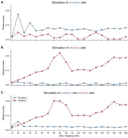
Figure S3 (Figure 2 – Figure Supplement 2).
Cell-intrinsic spiking activity in decoupled excitatory and inhibitory populations under ramping input. (A) Input-Frequency (I-F) curves for excitatory cells (left panel; pyramidal neurons with ICAN) and inhibitory cells (right panel; interneurons, fast-spiking) used in the model. Above a certain tonic input (around 0.35 nA for excitatory and 0.1 nA for inhibitory neurons), neurons can spike in the gamma range. (B) Raster plot showing the spiking activity of excitatory (blue, NE = 1000) and inhibitory (red, NI = 100) neurons in decoupled populations under ramping input (top trace) and in the absence of noise in the membrane potential. Despite random initial conditions across neurons, oscillations emerge in both populations due to the intrinsic properties of the cells, with a frequency that is predicted by the respective I-F curves (panel A.). (C) Similar representation as panel B. but with the addition of stochastic noise in the membrane potential of each neuron. The presence of noise disrupts the emergence of oscillations in these decoupled populations.
Author response image 5

Figure S6 (Figure 3 – Figure Supplement 2).
Quantification of PAC with and without noise. (A) Quantifying PAC in the absence of noise produced inaccurate identification of the coupled frequency bands, due to the complete absence of oscillations at some frequencies. All analyses are based on the CA1 firing rates (top traces) during a representative simulation. Power spectral densities of these firing rates (left) indicate that some frequencies have a power of 0. PAC of the excitatory population was assessed using two graphical representations, the polar plot (middle) and comodulogram (right), and quantified using the MI. The comodulogram was calculated by computing the MI across 80% overlapping 1-Hz frequency bands in the theta range and across 90% overlapping 10-Hz frequency bands in the gamma range and subsequently plotted as a heat map. In the absence of noise, a slow theta frequency centered around 5 Hz is found to modulate a broad range of gamma frequencies between 40 and 100 Hz. The value indicated on the comodulogram indicates the average MI in the 3-9 Hz theta range and 40-80 Hz gamma range. As in Figure 2, the polar plot represents the amplitude of gamma oscillations (averaged across all theta cycles) at each phase of theta (theta range: 3-9 Hz, phase indicated as angular coordinate) and for different gamma frequencies (radial coordinate, binned in 1-Hz ranges). (B) Adding uniform noise to the firing rate (with an amplitude ranging between 15 and 25% of the maximum firing rate) improved the identification of the coupled frequency bands. In this case, the slower theta frequency centered around 5 Hz modulates a gamma band located between 45 and 75 Hz.
Author response image 6

Figure S8 (Figure 3 – Figure Supplement 4).
A neural mass model of coupled excitatory and inhibitory neurons driven by Kuramoto oscillators generates theta-nested gamma oscillations and theta phase reset. (A) Two coupled neural masses (one excitatory and one inhibitory) driven by Kuramoto oscillators, which represent a dynamical oscillatory drive in the theta range, were used to implement a neural mass equivalent to our conductance-based model represented in Figure 1. Neural masses were modeled using the WilsonCowan formalism, with parameters adapted from Onslow et al. (2014) ( = 4.8, = = 4, = 0). (B) The normalized population firing rates exhibit theta-nested gamma oscillations (middle and bottom panels) in response to the dynamic theta rhythm (top panel). A stimulation pulse delivered at the descending phase of the rhythm to both populations (marked by the inverted red triangle) produces a robust theta phase reset, similarly to Figure 3A.
Author response image 7

Figure S12 (Figure 5 – Figure Supplement 4).
CAN currents are necessary for the production of selfsustained theta-gamma oscillations in response to single-pulse stimulation. (A) Same as Figure 5B. (B) Similar simulation as panel A., but without the presence of CAN currents in the EC, CA3 and CA1 fields of the hippocampus. Removing CAN currents from the model abolishes self-sustained theta-nested gamma oscillations in response to a single stimulation pulse (for the parameters represented in Figure 5, point B).
Author response image 8

On the figure below, we illustrate the phase response curves of CA3 neurons measured by Lengyel et al., 2005 (A), and compare it with our simulated phase response curves (B).
Note that the conventions for phase advance and phase delay are reversed between the two panels.
Author response image 9

Figure S7 (Figure 3 – Figure Supplement 3).
Network behavior generated by Kuramoto oscillators with nonphysiological phase response functions. Each panel is similar to Figure 3A, but with a different offset added to the phase response function of the Kuramoto oscillators (see methods, Equation 4). The center frequency was set to 6 Hz in all of these simulations. Overall, theta oscillations in these cases are less sinusoidal and show more abrupt phase changes than in the physiological case. (A) A phase offset of leads to an overall theta oscillation of 4 Hz, with a second peak following the main theta peak. (B) A phase offset of reduces the peak of theta, resetting the rhythm to the middle of the ascending phase. (C) A phase offset of or leads to the CA1 output resetting the theta rhythm to the trough of theta.
Author response image 10

Figure S3 (Figure 2 – Supplement 2).
Cell-intrinsic spiking activity in decoupled excitatory and inhibitory populations under ramping input. (A) Input-Frequency (I-F) curves for excitatory cells (left panel; pyramidal neurons with ICAN) and inhibitory cells (right panel; interneurons, fast-spiking) used in the model. Above a certain tonic input (around 0.35 nA for excitatory and 0.1 nA for inhibitory neurons), neurons can spike in the gamma range. (B) Raster plot showing the spiking activity of excitatory (blue, NE = 1000) and inhibitory (red, NI = 100) neurons in decoupled populations under ramping input (top trace) and in the absence of noise in the membrane potential. Despite random initial conditions across neurons, oscillations emerge in both populations due to the intrinsic properties of the cells, with a frequency that is predicted by the respective IF curves (panel A.). (C) Similar representation as panel B. but with the addition of stochastic noise in the membrane potential of each neuron. The presence of noise disrupts the emergence of oscillations in these decoupled populations.
Tables
Table 1
Full list of the default parameter values for the Kuramoto oscillators.
| Parameter | Value | |
|---|---|---|
| Number of oscillators () | 250 | |
| Center frequency () | 6 Hz | |
| Standard deviation () | 0.5 HZ | |
| Synchronization ratio () | 15 | |
| Phase reset gain () | 4 | |
| Peak phase () | 0 rad | |
| Firing rate time constant () | 10 ms | |
Table 2
Full list of parameter values and expressions for pyramidal neurons.
| Parameter | Expression |
|---|---|
Table 3
Full list of parameter values and expressions for interneurons.
| Parameter | Expression |
|---|---|
Table 4
A pre-synaptic spike causes an increase in the conductances and in the post-synaptic neuron.
The values for the intra-area connections are given here. Empty cells indicate no connection between the populations.
| E→E | E→I | I→E | I→I | |
|---|---|---|---|---|
| EC | 20 pS | 600 pS | ||
| DG | 180 pS | 1800 pS | ||
| CA3 | 20 pS | 20 pS | 600 pS | |
| CA1 | 60 pS | 1800 pS | 1800 pS |
Table 5
A pre-synaptic spike causes an increase in the conductances and in the post-synaptic neuron.
The values for the inter-area connections are given here. Empty cells indicate no connection between the areas. Recurrent projections are not allowed and are marked with dashes.
| Source | Target | |||
|---|---|---|---|---|
| EC | DG | CA3 | CA1 | |
| EC | - | 20 pS | 20 pS | 20 pS |
| DG | - | 180 pS | ||
| CA3 | - | 20 pS | ||
| CA1 | 60 pS | - | ||
Table 6
Number of neurons per subfield of the hippocampal formation, divided by neuron type.
| Area | ||
|---|---|---|
| EC | 10,000 | 1,000 |
| DG | 10,000 | 100 |
| CA3 | 1,000 | 100 |
| CA1 | 10,000 | 1,000 |
Table 7
Maximum probability of connection (, Equation 14) between neurons within each region.
| Py-Py | Py-Inh | Inh-Py | Inh-Inh | |
|---|---|---|---|---|
| EC | 0 | 0.37 | 0.54 | 0 |
| DG | 0 | 0.06 | 0.14 | 0 |
| CA3 | 0.56 | 0.75 | 0.75 | 0 |
| CA1 | 0 | 0.28 | 0.3 | 0.7 |
Table 8
Inter-area connection strengths ().
The source is always the excitatory population of the subfield. The same values are used when targeting excitatory and inhibitory populations. Empty cells indicate no connections. EC: Entorhinal Cortex, DG: Dentate Gyrus.
| Source | Target | |||
|---|---|---|---|---|
| EC | DG | CA3 | CA1 | |
| EC | - | 13.0 | 0.14 | 1.1 |
| DG | - | 0.14 | ||
| CA3 | - | 1.1 | ||
| CA1 | 0.2 | - | ||
Additional files
Download links
A two-part list of links to download the article, or parts of the article, in various formats.
Downloads (link to download the article as PDF)
Open citations (links to open the citations from this article in various online reference manager services)
Cite this article (links to download the citations from this article in formats compatible with various reference manager tools)
A dynamical computational model of theta generation in hippocampal circuits to study theta-gamma oscillations during neurostimulation
eLife 12:RP87356.
https://doi.org/10.7554/eLife.87356.3


