Figures and data in A three filament mechanistic model of musculotendon force and impedance

Figures
Tables
Additional files

18 figures, 6 tables and 1 additional file

Figures

Figure 1

Download asset Open asset

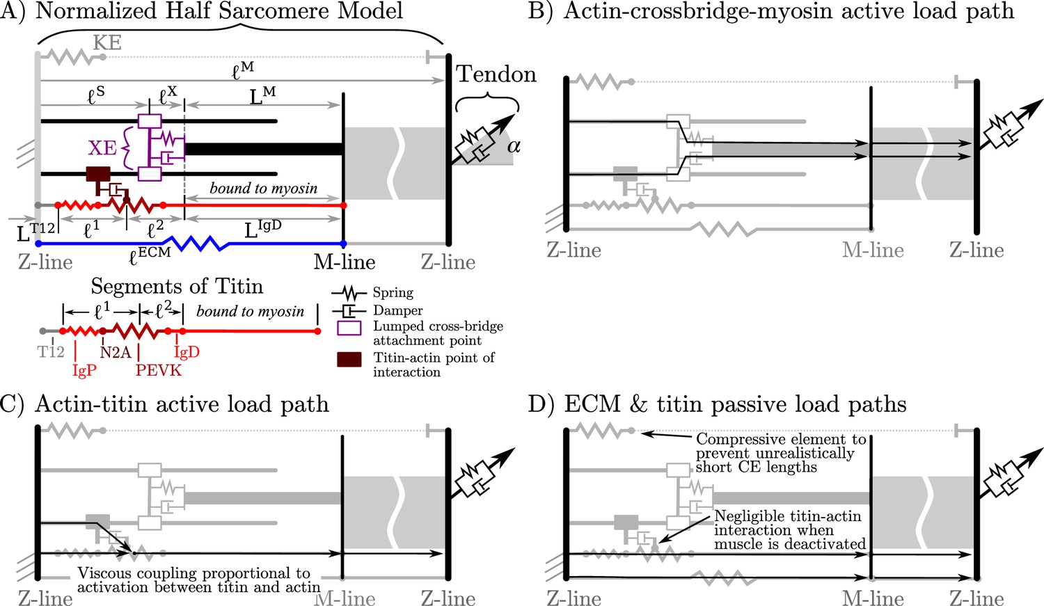
Overview of the VEXAT model and its components.

The name of the VEXAT model comes from the viscoelastic crossbridge and active titin elements (A) in the model. Active tension generated by the lumped crossbridge ﬂows through actin, myosin, and the adjacent sarcomeres to the attached tendon (B). Titin is modeled as two springs of length $l^{1}$ and $l^{2}$ in series with the rigid segments $L^{T12}$ and $L^{IgD}$ . Viscous forces act between titin and actin in proportion to the activation of the muscle (C), which reduces to negligible values in a purely passive muscle (D). We modeled actin and myosin as rigid elements; the XE, titin, and the tendon as viscoelastic elements; and the ECM as an elastic element.

Figure 2

Download asset Open asset

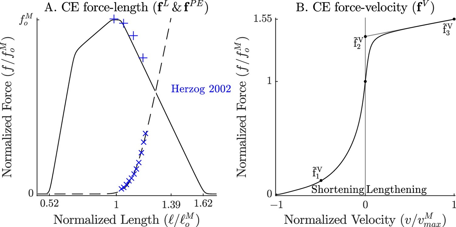
The force-length and force-velocity relations of the cat soleus model.

The model relies on Bézier curves to model the nonlinear effects of the active-force-length curve, the passive-force-length curve (A), and the force-velocity curve (B). Since nearly all of the reference experiments used in the ‘Biological benchmark simulations’ section have used cat soleus, we have fit the active-force-length curve ( $f^{L} (\cdot)$ ) and passive-force-length curves ( $f^{P E} (\cdot)$ ) to the cat soleus data of Herzog and Leonard, 2002. The concentric side of the force-velocity curve ( $f^{V} (\cdot)$ ) has been fitted to the cat soleus data of Herzog and Leonard, 1997.

Figure 3

Download asset Open asset

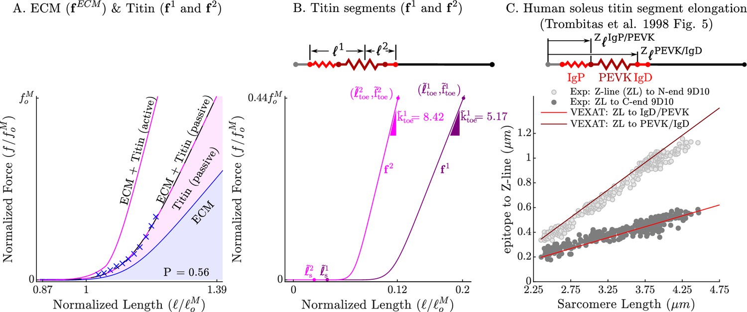
The passive force-length relations of the ECM, titin, and titin’s segments.

The passive force-length curve has been decomposed such that 56% of it comes from the ECM while 44% comes from titin to match the average of ECM-titin passive force distribution (which ranges from 43% to 76%) reported by Prado et al., 2005 (A). The elasticity of the titin segment has been further decomposed into two serially connected sections: the proximal section consisting of the T12, proximal IgP segment and part of the PEVK segment, and the distal section consisting of the remaining PEVK section and the distal Ig segment (B) The stiffness of the IgP and PEVK segments has been chosen so that the model can reproduce the movements of IgP/PEVK and PEVK/IgD boundaries that Trombitás et al., 1998b (C) observed in their experiments. The curves that appear in subplots A and B come from scaling the two-segmented human soleus titin model to cat soleus muscle. The curves that appear in subplot C compare the human soleus titin model’s IgP, PEVK, and IgD force-length relations to the data of Trombitás et al., 1998b (see in Appendix 2 for details).

Figure 4

Download asset Open asset

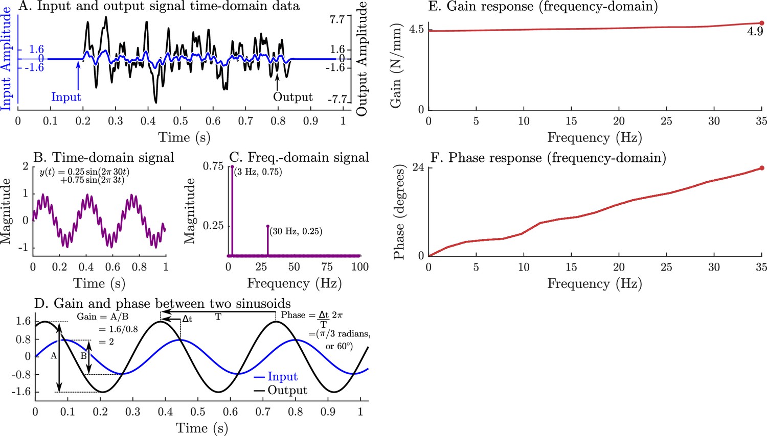
A graphical overview of a system’s response in the time-domain, frequency-domain, its gain-response, and its phase-response.

Evaluating a system’s gain and phase response begins by applying a pseudo-random input signal to the system and measuring its output (A). Both the input and output signals (A) are transformed into the frequency domain by expressing these signals as an equivalent sum of scaled and shifted sinusoids (simple example shown in B and C). Each individual input sinusoid is compared with the output sinusoid of the same frequency to evaluate how the system scales and shifts the input to the output (D). This process is repeated across all sinusoid pairs to produce a function that describes how an input sinusoid is scaled (E) and shifted (F) to an output sinusoid using only the measured data (A).

Figure 5

Download asset Open asset

The time-domain and power-spectrum of the bandwidth-limited stochastic perturbation signals.

The perturbation waveforms are constructed by generating a series of pseudo-random numbers, padding the ends with zeros, by ﬁltering the signal using a 2nd order low-pass ﬁlter (wave forms with –3 dB cut-off frequencies of 90 Hz, 35 Hz, and 15 Hz appear in A) and ﬁnally by scaling the range to the desired limit (1.6 mm in A). Although the power spectrum of the resulting signals is highly variable, the ﬁlter ensures that the frequencies beyond the –3 dB point have less than half their original power (B).

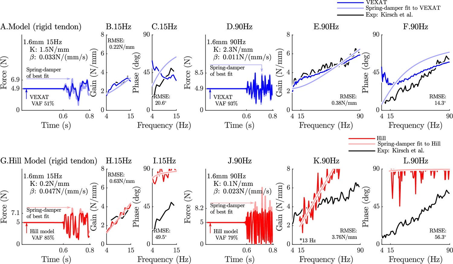
Figure 6

Download asset Open asset

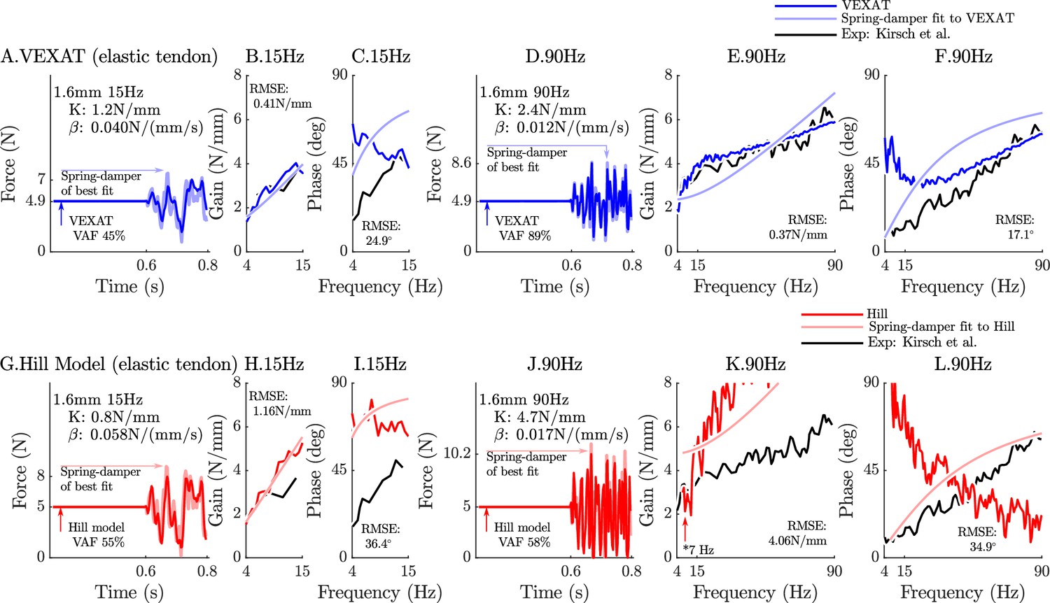
The response of the elastic-tendon models (VEXAT and Hill) to the 15Hz and 90Hz perturbations.

The 15 Hz perturbations show that the VEXAT model’s performance is mixed: in the time-domain (A.) the VAF is lower than the 78–99% analyzed by Kirsch et al., 1994; the gain response (B.) follows the proﬁle in Figure 3 of Kirsch et al., 1994, while the phase response differs (C.). The response of the VEXAT model to the 90 Hz perturbations is much better: a VAF of 91% is reached in the time-domain (D.), the gain response follows the response of the cat soleus analyzed by Kirsch et al., 1994, while the phase-response follows biological muscle closely for frequencies higher than 30 Hz. Although the Hill’s time-domain response to the 15 Hz signal has a higher VAF than the VEXAT model (G.), the RMSE of the Hill model’s gain response (H.) and phase response (I.) shows it to be more in error than the VEXAT model. While the VEXAT model’s response improved in response to the 90 Hz perturbation, the Hill model’s response does not: the VAF of the time-domain response remains low (J.), neither the gain (K.) nor phase responses (L.) follow the data of Kirsch et al., 1994. Note that the Hill model’s 90 Hz response was so nonlinear that the lowest frequency analyzed had to be raised from 4 Hz to 7 Hz to satisfy the criteria that $(C_{x y})^{2} \geq 0.67$ .

Figure 7

Download asset Open asset

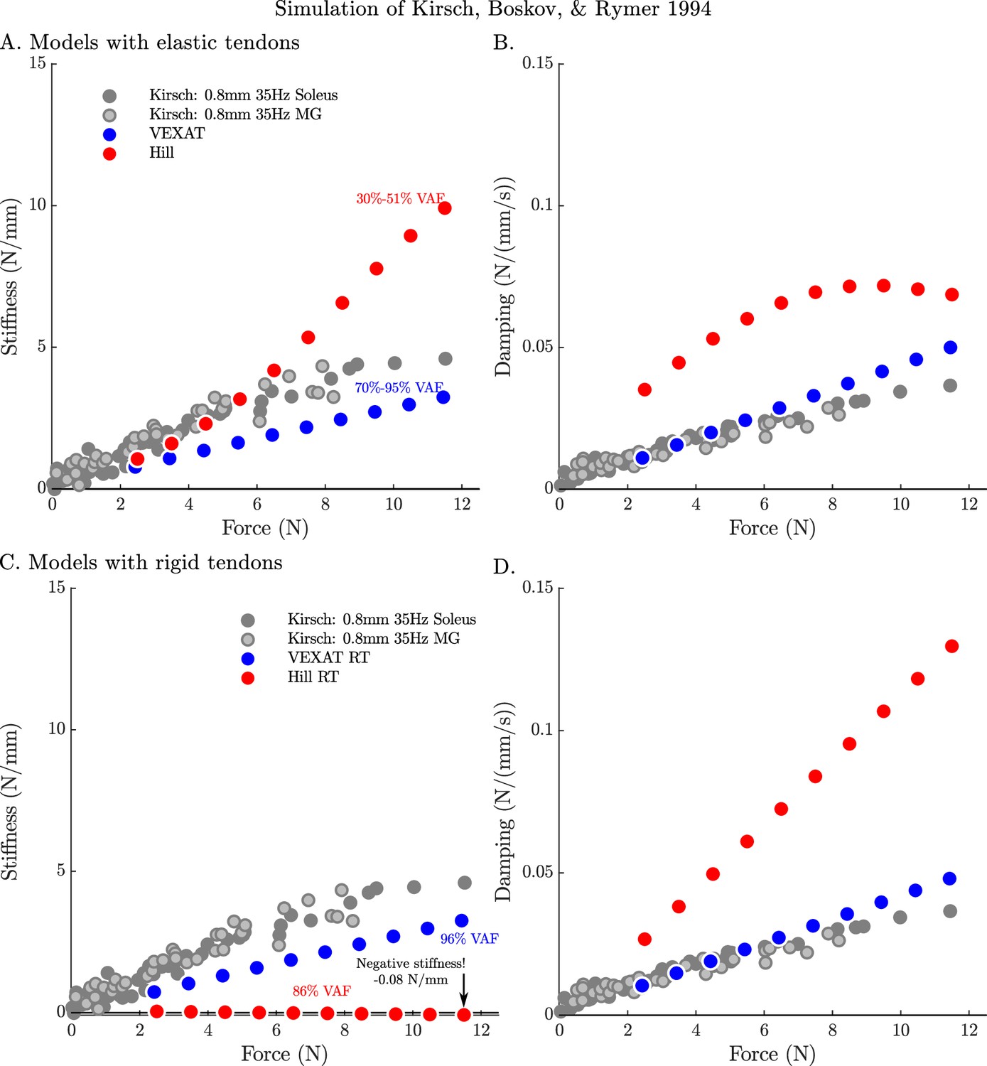
The stifffness-force and damping-force (impedance-force) relations of the models when coupled with elastic and rigid tendons.

When coupled with an elastic-tendon, the stiffness (A) and damping (B) coefficients of best ﬁt of both the VEXAT model and a Hill model increase with the tension developed by the MTU. However, both the stiffness and damping of the elastic-tendon Hill model are larger than Kirsch et al.’s coefficients (from Figure 12 of Kirsch et al., 1994), particularly at higher tensions. When coupled with rigid-tendon the stiffness (C) and damping (D) coefficients of the VEXAT model remain similar, as the values for $k_{o}^{X}$ and $β_{o}^{X}$ have been calculated to take the tendon model into account (see Appendix 2.5 for details). In contrast, the stiffness and damping coefficients of the rigid-tendon Hill model differ dramatically from the elastic-tendon Hill model: while the elastic-tendon Hill model is too stiff and damped, the rigid-tendon Hill model is not stiff enough (compare A. to C.) and far too damped (compare B. to D.). Coupling the Hill model with a rigid-tendon increases the VAF from 30–51% to 86% but this improved accuracy is made using stiffness and damping that deviates from that of biological muscle (Kirsch et al., 1994).

Figure 8

Download asset Open asset

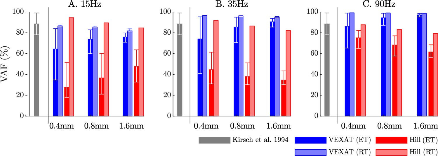
The VAF of each model varies systematically with the type of model, perturbation amplitude, frequency, and the nominal tension.

Kirsch et al., 1994 noted that the spring-damper model of best ﬁt has a VAF of between 78–99% across all experiments. We have repeated the perturbation experiments to evaluate the VAF across a range of conditions: two different tendon models, three perturbation bandwidths (15 Hz, 35 Hz, and 90 Hz), three perturbation magnitudes (0.4 mm, 0.8 mm, and 1.6 mm), and ten nominal force values (spaced evenly between 2.5 N and 11.5 N). Each bar in the plot shows the mean VAF across all 10 nominal force values, with the whiskers extending to the minimum and maximum value that occurred in each set. The mean VAF of the VEXAT model changes by up to 36% depending on the condition, with the lowest mean VAF occurring in response to the 0.4mm 15 Hz perturbation with an elastic-tendon (A), and the highest mean VAF occurring in response to the 90 Hz perturbations with the rigid-tendon (C). In contrast, the mean VAF of the Hill model varies by up to 67% depending on the condition, with the lowest VAF occurring in the 15 Hz 0.4 mm trial with the elastic-tendon (A), and the highest value VAF occurring in the 15 Hz 0.4 mm trial with the rigid-tendon (A).

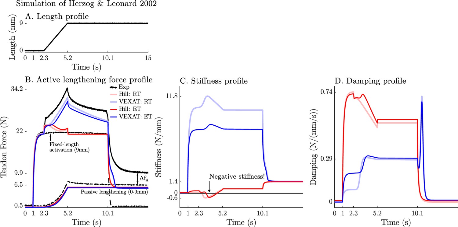
Figure 9

Download asset Open asset

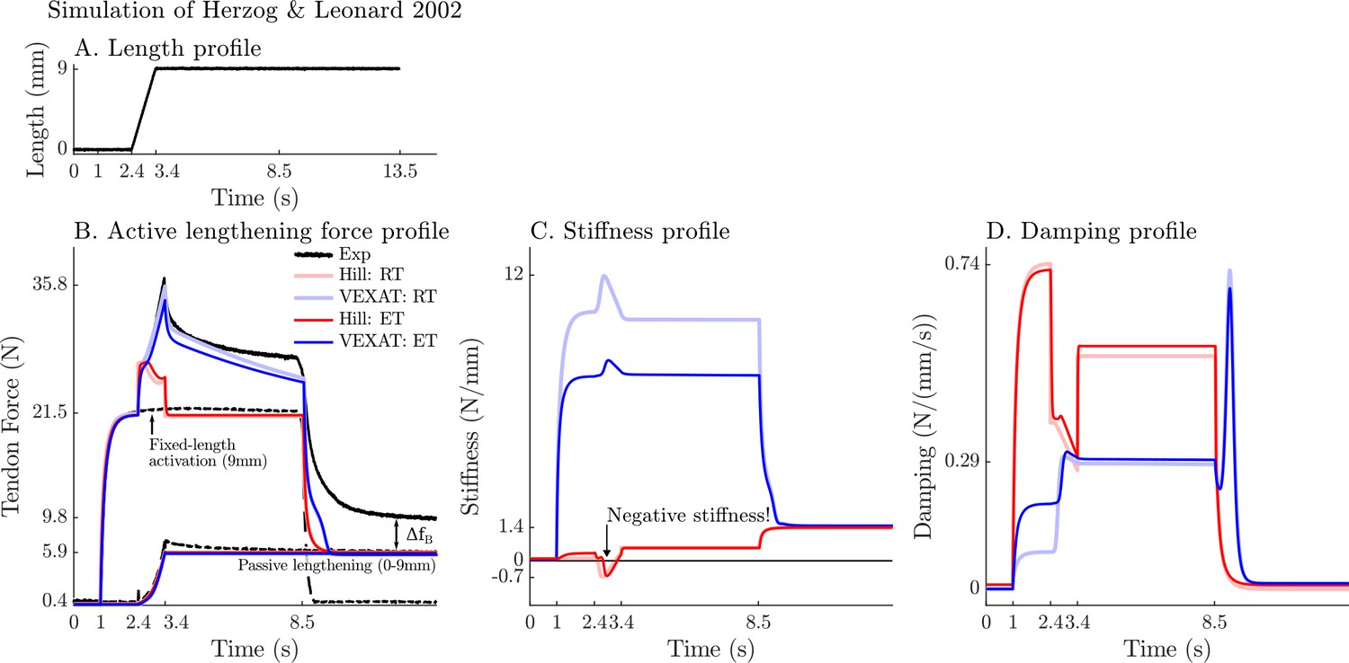
A comparison of the tension developed by the VEXAT and Hill models when actively lengthened at 9 mm/s on the descending limb of the force-length relation.

Herzog and Leonard, 2002 actively lengthened (A) cat soleus muscles on the descending limb of the force-length curve (where ${\tilde{l}}^{M} > 1$ in Figure 2A) and measured the force response of the MTU (B). After the initial transient at 2.4s the Hill model’s output force drops (B) because of the small region of negative stiffness (C) created by the force-length curve. In contrast, the VEXAT model develops steadily increasing forces between 2.4 and 3.4s and has a consistent level of stiffness (C) and damping (D).

Figure 10

Download asset Open asset

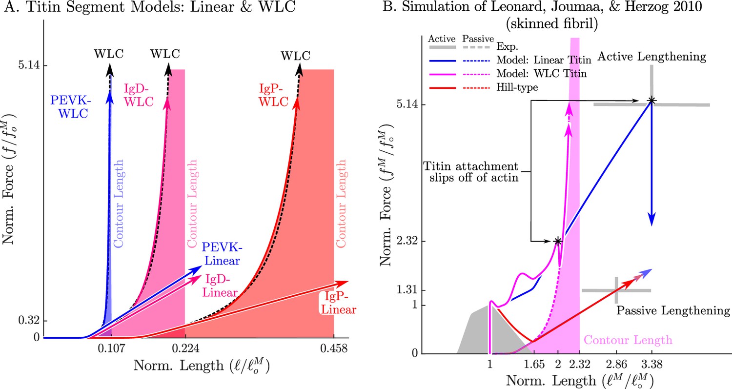
The passive force-length relations of two diffferent models of titin: a linear extrapolation and a WLC model.

We consider two different versions of the force-length relation for each titin segment of the VEXAT model (A): a linear extrapolation, and a WLC model extrapolation. Leonard et al., 2010 observed that active myoﬁbrils continue to develop increasing amounts of tension beyond actin-myosin overlap (B, grey lines with ±1 standard deviation shown). When this experiment is replicated using the VEXAT model (B, blue & magenta lines) and a Hill model (C red lines), only the VEXAT model with the linear extrapolated titin model is able to replicate the experiment with the titin-actin bond slipping off of the actin ﬁlament at 3.38 $l_{o}^{M}$ .

Figure 11

Download asset Open asset

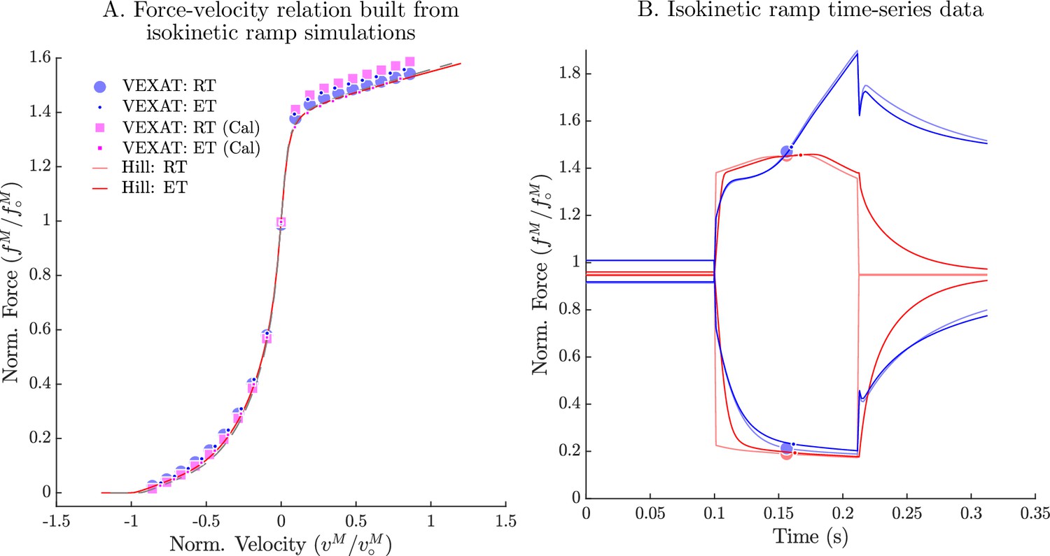
The force-velocity relation of the VEXAT and Hill models.

When the experiments of Hill, 1938 are simulated (A), the VEXAT model produces a force-velocity proﬁle (blue dots) that approaches zero more rapidly during shortening than the embedded proﬁle $f^{V} (\cdot)$ (red lines). By scaling $v_{m a x}^{M}$ by 0.95 the VEXAT model (magenta squares) is able to closely follow the force-velocity curve of the Hill model. While the force-velocity curves between the two models are similar, the time-domain force response of the two models differs substantially (B). The rigid-tendon Hill model exhibits a sharp nonlinear change in force at the beginning (0.1 s) and ending (0.21 s) of the ramp stretch.

Figure 12

Download asset Open asset

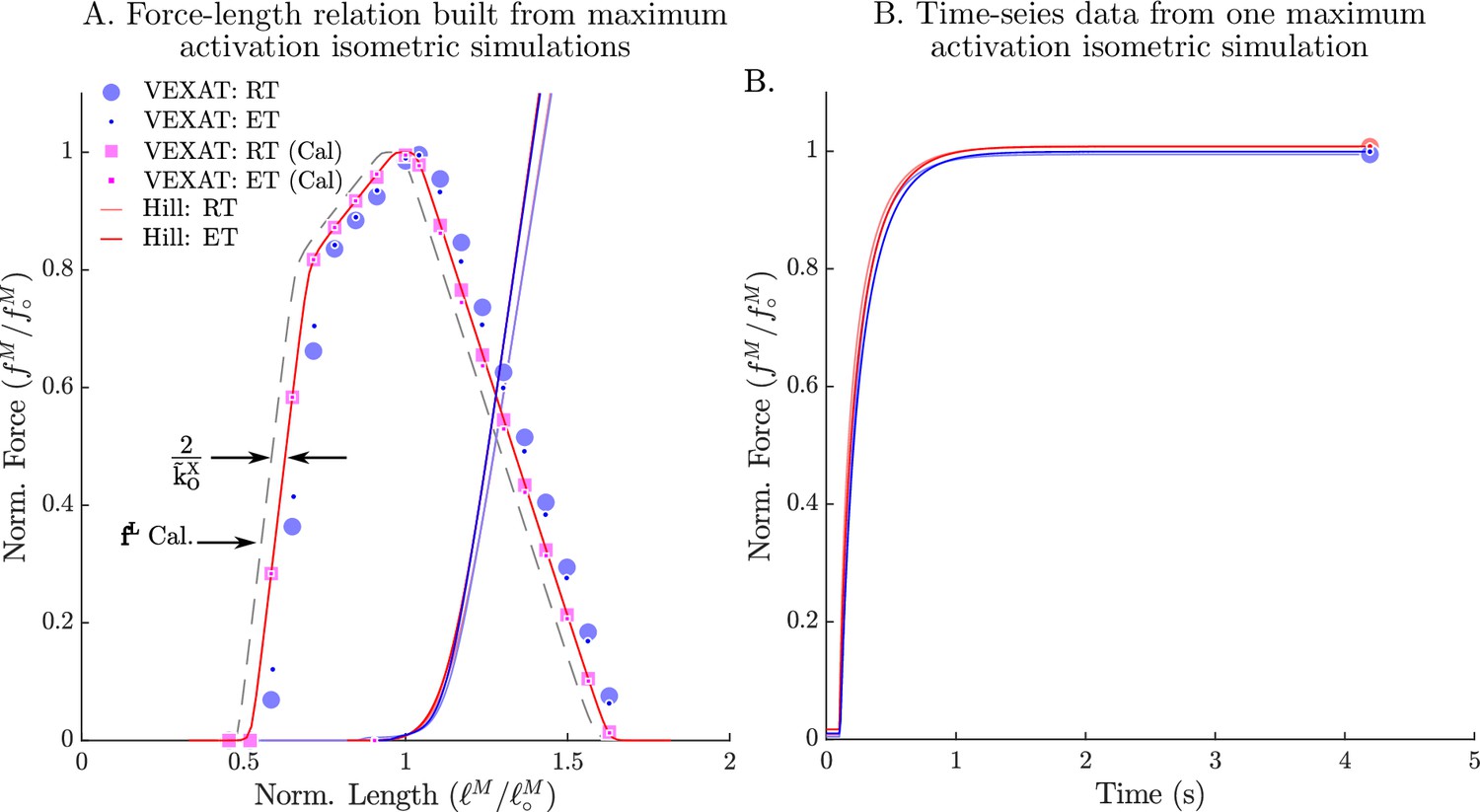
The passive and active force-length relation of the VEXAT and Hill models.

When the passive and active force-length experiments of Gordon et al., 1966 are simulated, the VEXAT model (blue dots) and the Hill model (red lines) produce slightly different force-length curves (A) and force responses in the time-domain (B). The VEXAT model produces a right shifted active force-length curve, when compared to the Hill model due to the series elasticity of the XE element. By shifting the underlying curve by $\frac{2}{k_{o}^{X}}$ to the left the VEXAT model (magenta squares) can be made to exactly match the force-length characteristic of the Hill model.

Appendix 1—figure 1

Download asset Open asset

The average point of attachment between myosin and actin in a half-sarcomere at the optimal length.

To evaluate the stiﬀness of the actin-myosin load path, we ﬁrst determine the average point of attachment. Since the actin ﬁlament length varies across species we label it $L^{A}$ . Across rabbits, cats and human skeletal muscle myosin geometry is consistent Rassier et al., 1999: a half-myosin is 0.8 μm in length with a 0.1 μm bare patch in the middle. Thus at full overlap the average point of attachment is 0.45 μm from the M-line, or $L^{A}$ − 0.45 μm from the Z-line at $l_{o}^{M}$ . The lumped stiffness of the actin-myosin load path of a half-sarcomere is the stiﬀness of three springs in series: a spring representing a $L^{A}$ − 0.45 μm length of actin, a spring representing the all attached crossbridges, and a spring representing a 0.45 μm section of myosin.

Appendix 1—figure 2

Download asset Open asset

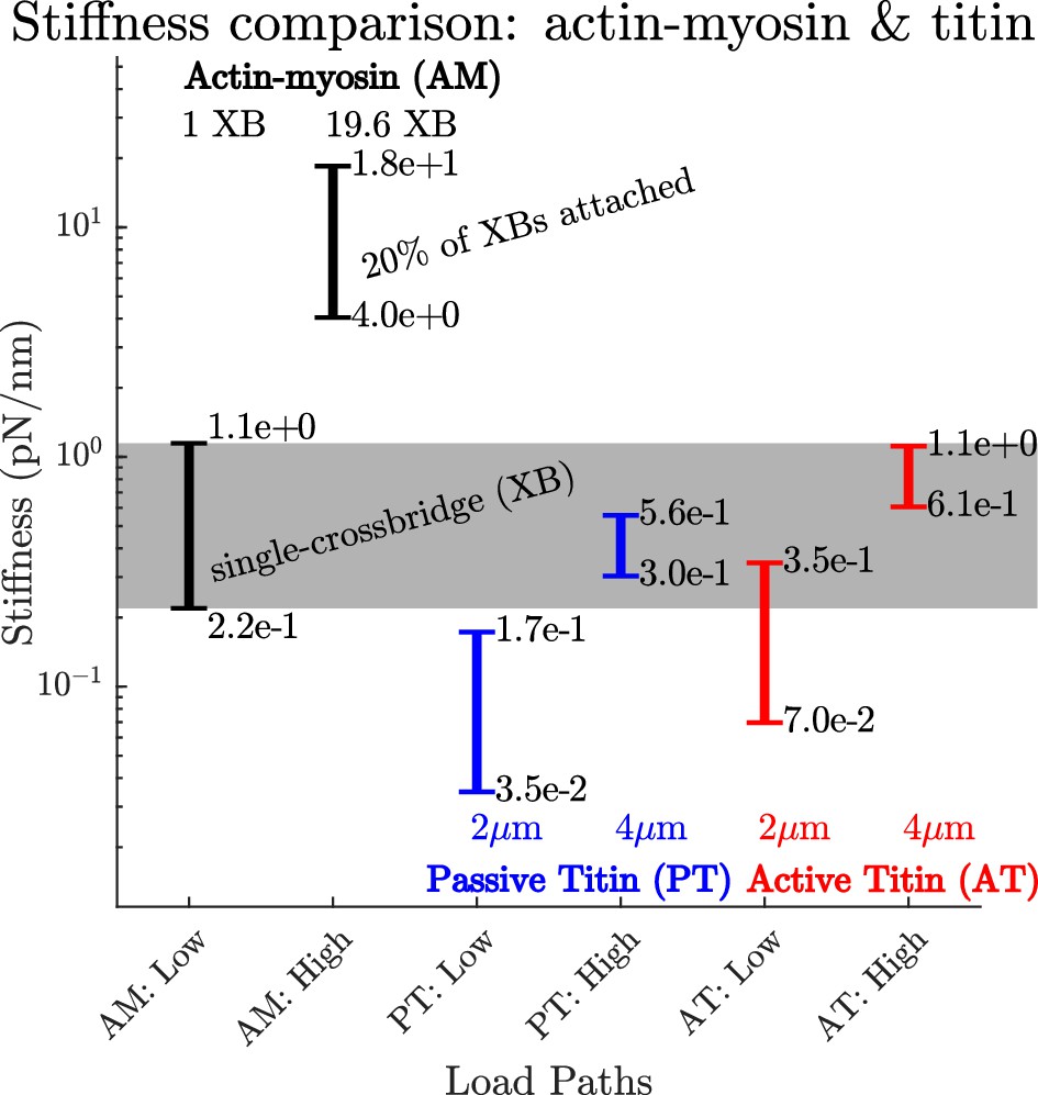
A comparison of how actin-myosin and titin’s stiffness varies.

The stiffness of a rabbit’s actin-myosin load path with a single attached crossbridge (1 XB) exceeds the stiffness of its titin ﬁlament at lengths of 2μm ( $1.62 l_{o}^{M}$ ) (compare AM:Low to PT:Low and PT:High). Only when titin is stretched to 4μm ( $3.25 l_{o}^{M}$ ) does its stiffness (PT:High and AT:High) become comparable to the actin-myosin with a single attached crossbridge (AM:Low). At higher activations and modest lengths, the stiffness of the actin-myosin load path (AM: High) exceeds the stiffness of titin (PT: Low and AT:Low) by between two and three orders of magnitude. At higher activations and longer lengths, the stiffness of the actin-myosin load path (AM: High) exceeds the stiffness of titin by roughly an order of magnitude (PT:High and AT:High).

Appendix 2—figure 1

Download asset Open asset

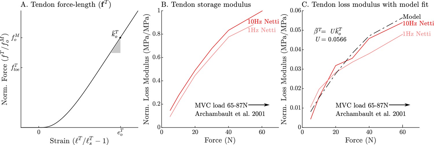
The models used to define the force, storage modulus, and loss modulus of tendon.

The normalized tendon force-length curve (A) has been been ﬁt to match the cat soleus tendon stiffness measurements of Scott and Loeb, 1995. The data of Netti et al., 1996 allow us to develop a model of tendon damping as a linear function of tendon stiffness. By normalizing the measurements of Netti et al., 1996 by the maximum storage modulus we obtain curves that are equivalent to the normalized stiffness (B) and damping (C) of an Achilles tendon from a rabbit. Both normalized tendon stiffness and damping follow similar curves, but at different scales, allowing us to model tendon damping as a linear function of tendon stiffness (C).

Appendix 6—figure 1

Download asset Open asset

The response of the rigid-tendon models (VEXAT and Hill) to the 15Hz and 90Hz perturbations.

When coupled with a rigid-tendon, the VEXAT model’s VAF (A), gain response (B), and phase response (C) more closely follows the data of Figure 3 from Kirsch et al., 1994 than when an elastic-tendon is used. This improvement in accuracy is also observed at the 90 Hz perturbation (**D, E, and F**), though the phase response of the model departs from the data of Kirsch et al., 1994 for frequencies lower than 30 Hz. Parts of the Hill model’s response to the 15 Hz perturbation are better with a rigid-tendon, with a higher VAF (G), a lower RMSE gain-response (H). but have a poor phase-response (I). In response to the higher frequency perturbations, the Hill model’s response is poor with an elastic (see Figure 6) or rigid-tendon. The VAF in response to the 90 Hz perturbation remains low (J), and neither the gain (K) nor the phase response of the Hill model (L) follow the data of Kirsch et al., 1994. The rigid-tendon Hill model’s nonlinearity was so strong that the lowest frequency analyzed had to be raised from 4 Hz to 21 Hz to meet the criteria that $(C_{x y})^{2} \geq 0.67$ .

Appendix 7—figure 1

Download asset Open asset

The response of the VEXAT and Hill models to active lengthening on the descending limb at 3 mm/s.

Simulation results of the 3 mm/s (A) active lengthening experiment of Herzog and Leonard, 2002 (B). As with the 9 mm/s trial, the Hill model’s force response drops during the ramp due to a small region of negative stiffness introduced by the descending limb of the force-length curve (C), and a reduction in damping (D) due to the ﬂattening of the force-velocity curve. Note: neither model was ﬁtted to this trial.

Appendix 7—figure 2

Download asset Open asset

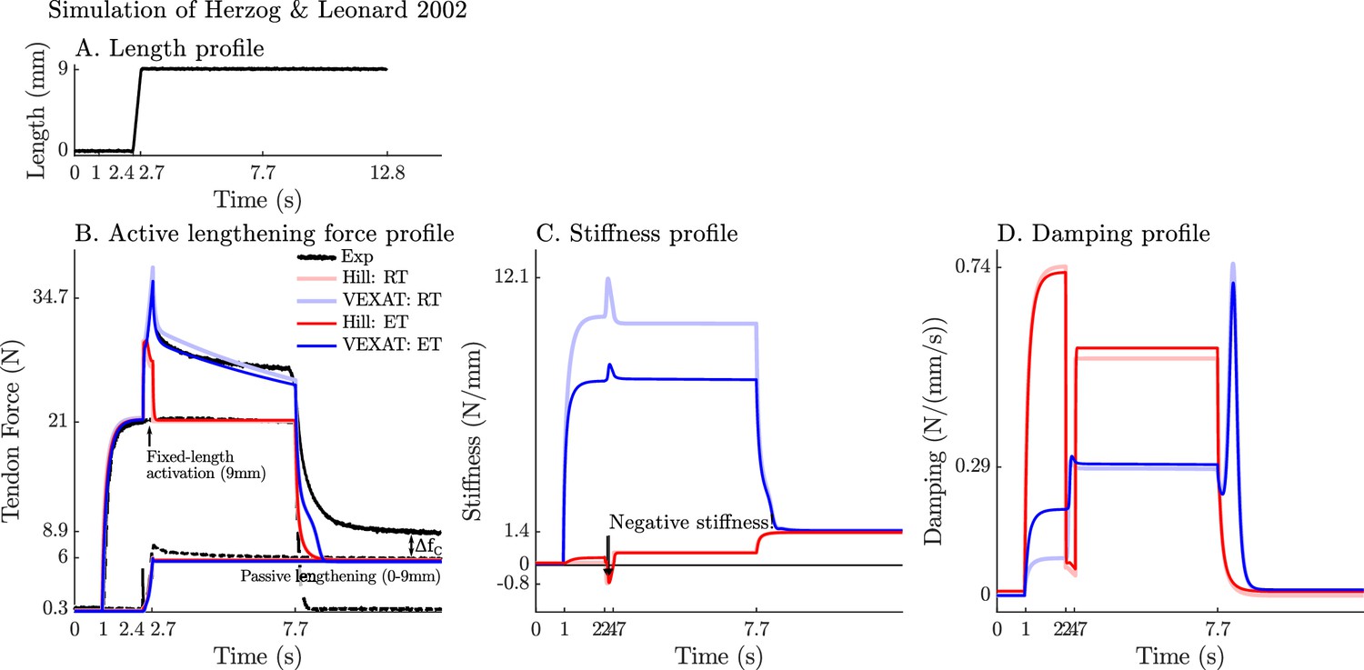
The response of the VEXAT and Hill models to active lengthening on the descending limb at 27 mm/s.

Simulation results of the 27 mm/s (A) active lengthening experiment of Herzog and Leonard, 2002 (B). As with the prior simulations the Hill model exhibits a small region of negative stiffness introduced by the descending limb of the force-length curve (C) and a drop in damping (D). Note: neither model was ﬁtted to this trial.

Tables

Table 1

The VEXAT and Hill model’s elastic-tendon cat soleus MTU parameters.

The VEXAT model uses all of the Hill model’s parameters which are highlighted in grey. Short forms are used to indicate: length ‘len’, velocity ‘vel’, acceleration ‘acc’, half ‘h’, activation ‘act’, segment ‘seg’, threshold ‘thr’, and stiffness ‘stiff’. The letters ‘R’ or ‘H’ in front of a reference mean the data is from a rabbit or a human, otherwise the data is from cat soleus. References are in brackets and are coded in order of appearance as: ‘H02’ for Herzog and Leonard, 2002, ‘S82’ for Sacks and Roy, 1982, ‘S96’ for Scott et al., 1996, ‘H38’ for Hill, 1938, ‘S95’ for Scott and Loeb, 1995, ‘N96’ for Netti et al., 1996, ‘R99’ for Rassier et al., 1999, ‘K94’ for Kirsch et al., 1994, ‘P05’ for Prado et al., 2005, and ‘T98’ for Trombitás et al., 1998b. The letters following a reference indicate how the data was used to create the parameter: ‘C’ calculated, ‘F’ fit, ‘E’ estimated, or ‘S’ scaled. Most of the VEXAT model’s XE and titin parameters can be used as rough parameter guesses for other muscles because we have expressed these parameters in a normalized space: the values will scale appropriately with changes to $l_{o}^{M}$ and $f_{o}^{M}$ . Titin’s force-length curves, however, should be updated if $N^{IgP}$ , $N^{PEVK}$ , or $N^{IgD}$ differ from the values shown below (see Appendix 2 for details). Note that the rigid-tendon cat soleus parameters differ from the table below because tendon elasticity affects the fitting of ${\tilde{k}}_{o}^{X}$ , ${\tilde{β}}_{o}^{X}$ , $f^{PE}$ , $f^{1} ({\tilde{l}}^{1})$ , and $f^{2} ({\tilde{l}}^{2})$ . Finally, the parameters related to the compressive element (F), the XE (G), and titin (H and I) can be used as initial values when simulating the MTU’s other mammals. By making use of these defaults, the VEXAT model requires the same number of parameters as a Hill-type muscle model (A—E).

Parameter		Value	Source
A. Basic parameters
Max iso force	$f_{o}^{M}$	$21.5 N$	(H02)F
Opt CE len	$l_{o}^{M}$	$42.9 mm$	(H02)F
Pen angle	$α$	${7.00}^{\circ}$	(S82)
Act time const	$τ_{A}$	$113 ms$	(H02)F
De-act time const	$τ_{D}$	$142 ms$	(H02)F
B. Force-velocity relation: $f^{V} ({\hat{v}}^{M})$
Max shortening vel	$v_{max}^{M}$	$4.65 \frac{l_{o}^{M}}{s}$	(S96)F
$f^{V}$ at $- \frac{1}{2} v_{m a x}^{M}$	${\tilde{f}}_{1}^{V}$	$0.126 f_{o}^{M}$	(S96)F
$f^{V}$ at ${\hat{v}}^{M} = + 0$	${\tilde{f}}_{2}^{V}$	$1.40 f_{o}^{M}$	(H02)F
$f^{V}$ at $v_{m a x}^{M}$	${\tilde{f}}_{3}^{V}$	$1.55 f_{o}^{M}$	(H02)E
$v_{max}^{M}$ scaling	$s^{V}$	$0.950$	(H38)F
C. Tendon model: $f^{T} ({\tilde{l}}^{T})$ , $U {\hat{k}}^{T} ({\tilde{l}}^{T})$
Slack len	$l_{s}^{T}$	$30.5 mm$	(S95)S
Stiffness	${\tilde{k}}_{o}^{T}$	$30.0 \frac{f_{o}^{M}}{l_{s}^{T}}$	(S95)
Strain at $f_{o}^{M}$	$e_{o}^{T}$	$0.0458$	(S95)
Toe force	$f_{toe}^{T}$	$\frac{2}{3} f_{o}^{M}$	(S95)E
Damping	$U$	$0.057 s$	R(N96)F
D. Active force-length relation: $f^{L} ({\tilde{l}}^{M})$
Opt sarcomere len	$L_{\circ}^{M}$	$2.43 μ m$	(R99)
Actin len	${\tilde{L}}^{A}$	$0.462 l_{o}^{M}$	(R99)
Myosin h-len	${\tilde{L}}^{M}$	$0.330 l_{o}^{M}$	(R99)
Myosin bare h-len	${\tilde{L}}^{B}$	$0.0175 l_{o}^{M}$	(R99)
Offset	$Δ^{L}$	$- \frac{2}{{\tilde{k}}_{o}^{X}} l_{o}^{M}$	C
E. Passive force-length relation: $f^{PE} ({\tilde{l}}^{M})$
Slack len	${\tilde{l}}_{s}^{PE}$	$0.872 l_{o}^{M}$	(H02)F
Toe len	${\tilde{l}}_{toe}^{PE}$	$1.39 l_{o}^{M}$	(H02)F
Toe force	${\tilde{f}}_{toe}^{PE}$	$1.00 f_{o}^{M}$	(H02)F
Toe stiffness	${\tilde{k}}_{toe}^{PE}$	$3.88 \frac{f_{o}^{M}}{l_{o}^{M}}$	(H02)F
F. Compressive force-length relation: $f^{KE} ({\tilde{l}}^{M})$
Slack len	${\tilde{l}}_{s}^{PE}$	$\frac{1}{10} l_{o}^{M}$	E
Toe len	${\tilde{l}}_{toe}^{PE}$	$0.00 l_{o}^{M}$	E
Toe force	${\tilde{f}}_{toe}^{PE}$	$1.00 f_{o}^{M}$	E
G. XE viscoelastic model
Stiffness	${\tilde{k}}_{o}^{X}$	$49.1 \frac{f_{o}^{M}}{l_{o}^{M}}$	(K94)F:Figure 12
Damping	${\tilde{β}}_{o}^{X}$	$0.347 \frac{f_{o}^{M}}{l_{o}^{M} / s}$	(K94)F:Figure 12
Acc. time const	$τ^{S}$	$1.00 e- 3 s$	(K94,H38)E
Num acc damping	$D$	$1.00$	(K94,H39)E
Low act threshold	$a_{L}$	$0.0500$	(K94,H39)E
Len tracking gain	$G_{L}$	$1000 \frac{1}{s}$	(K94,H39)E
Vel tracking gain	$G_{V}$	$1000$	(K94,H39)E
H. Titin & ECM Parameters
ECM fraction	$P$	56%	R(P05)
PEVK attach pt	$Q$	$0.625$	(H02)F
Z-line–T12 len	${\tilde{L}}^{T12}$	$0.0412 l_{o}^{M}$	H(T98)
IgD rigid h-len	${\tilde{L}}^{IgD}$	${\tilde{L}}^{M}$	(R99)
No IgP domains	$N^{IgP}$	$60.5$	H(T98)S
No PEVK residues	$N^{PEVK}$	$1934.7$	H(T98)S
No IgD domains	$N^{IgD}$	$19.5$	H(T98)S
Active damping	$β_{A}^{PEVK}$	$71.9 \frac{f_{o}^{M}}{l_{o}^{M}}$	(H02)F
Passive damping	$β_{P}^{PEVK}$	$0.1 \frac{f_{o}^{M}}{l_{o}^{M}}$	E
Length threshold	${\tilde{l}}_{s}^{M}$	$\frac{1}{2} {\tilde{l}}_{s}^{PE}$	E
Act threshold	$A_{\circ}$	$0.05$	E
Step transition	$R$	$0.01$	E

I. Titin’s force-length relations: $f^{1} ({\tilde{l}}^{1})$ & $f^{2} ({\tilde{l}}^{2})$
$f^{1} ({\tilde{l}}^{1})$ slack len	${\tilde{l}}_{S}^{1}$	$0.0739 l_{o}^{M}$	H(T98)S, (H02)F
$f^{1} ({\tilde{l}}^{1})$ toe len	${\tilde{l}}_{toe}^{1}$	$0.1590 l_{o}^{M}$	H(T98)S, (H02)F
$f^{1} ({\tilde{l}}^{1})$ toe force	${\tilde{f}}_{toe}^{1}$	$(1 - P) f_{o}^{M}$	H(T98)S, (H02)F
$f^{1} ({\tilde{l}}^{1})$ toe stiff	${\tilde{k}}_{toe}^{1}$	$5.17 \frac{f_{o}^{M}}{l_{o}^{M}}$	H(T98)S, (H02)F
$f^{2} ({\tilde{l}}^{2})$ slack len	${\tilde{l}}_{S}^{2}$	$0.0454 l_{o}^{M}$	H(T98)S, (H02)F
$f^{2} ({\tilde{l}}^{2})$ toe len	${\tilde{l}}_{toe}^{2}$	$0.0977 l_{o}^{M}$	H(T98)S, (H02)F
$f^{2} ({\tilde{l}}^{2})$ toe force	${\tilde{f}}_{toe}^{2}$	$(1 - P) f_{o}^{M}$	H(T98)S, (H02)F
$f^{2} ({\tilde{l}}^{2})$ toe stiff	${\tilde{k}}_{toe}^{2}$	$8.42 \frac{f_{o}^{M}}{l_{o}^{M}}$	H(T98)S, (H02)F

Appendix 2—table 1

The relations that define how titin’s segments lengthen as a sarcomere is passively stretched.

The coefficients of the normalized lengths of ${\tilde{l}}^{I g P} ({\tilde{l}}^{M})$ , ${\tilde{l}}^{P E V K} ({\tilde{l}}^{M})$ , ${\tilde{l}}^{I g D} ({\tilde{l}}^{M})$ and from Equation 53-Equation 55 under passive lengthening. These coefficients (human soleus column) have been extracted from data of Figure 5 of Trombitás et al., 1998b using a least-squares ﬁt. Since Figure 5 of Trombitás et al., 1998b plots the change in segment length of a single titin ﬁlament against the change in length of the entire sarcomere, the resulting slopes are in length normalized units. The slopes sum to 0.5, by construction, to reﬂect the fact that these three segments of titin stretch at half the rate of the entire sarcomere (assuming symmetry). The cat soleus titin segment coefficients have been formed using a simple scaling of the human soleus titin segment coefficients, and so, are similar. Rabbit psoas titin geometry (Prado et al., 2005) differs dramatically from human soleus titin (Trombitás et al., 1998b) and produce a correspondingly large difference in the coefficients that describe the length of the segments of rabbit psoas titin.

Coefficient	Human	Feline	Rabbit
	Soleus Trombitás et al., 1998a	Soleus	Psoas
$A^{IgP}$	0.177	0.177	0.262
$b^{IgP}$	–0.101	–0.113	–0.189
$A^{PEVK}$	0.266	0.266	0.122
$b^{PEVK}$	–0.197	–0.221	–0.100
$A^{IgD}$	0.057	0.057	0.115
$b^{IgD}$	–0.033	–0.033	–0.083

Appendix 2—table 2

Normalized titin and crossbridge parameters ﬁt to data from the literature.

Symbol	Value	Unit	Source
${\tilde{k}}^{Ti}$	3.88	$f_{o}^{M} / l_{o}^{M}$	Herzog and Leonard, 2002
			Prado et al., 2005
${\tilde{k}}^{1}$	5.17	$f_{o}^{M} / l_{o}^{M}$	Trombitás et al., 1998b
${\tilde{k}}^{2}$	8.42	$f_{o}^{M} / l_{o}^{M}$	Trombitás et al., 1998b
${\tilde{k}}_{o}^{X}$	74.5	$f_{o}^{M} / (l_{o}^{M})$	Kirsch et al., 1994 (Figure 3)
${\tilde{β}}_{o}^{X}$	0.155	$f_{o}^{M} / (l_{o}^{M} / s)$	Kirsch et al., 1994 (Figure 3)
${\tilde{k}}_{o}^{X}$	49.1	$f_{o}^{M} / (l_{o}^{M})$	Kirsch et al., 1994 (Figure 12)
${\tilde{β}}_{o}^{X}$	0.347	$f_{o}^{M} / (l_{o}^{M} / s)$	Kirsch et al., 1994 (Figure 12)

Appendix 5—table 1

Mean normalized stiffness coefficients (A.), mean normalized damping coeffcients (B.), VAF (C.), and the bandwidth (D.) of linearity (coherence squared >0.67) for models with elastic-tendons.

Here, the proposed model has been ﬁtted to Figure 12 of Kirsch et al., 1994, while the experimental data from Kirsch et al., 1994 comes from Figures 9 and 10. Experimental data from Figure 12 of Kirsch et al., 1994 has not been included in this table because it would only contribute 1 entry and would overwrite values from Figures 9 and 10. The impedance experiments at each combination of perturbation amplitude and frequency have been evaluated at 10 different nominal forces linearly spaced between 2.5 N and 11.5 N. The results presented in the table are the mean values of these ten simulations. The VAF is evaluated between the model and the spring-damper of best ﬁt, rather than to the response of biological muscle (which was not published by Kirsch et al., 1994). Finally, model values for the VAF (C.) and the bandwidth of linearity (D.) that are worse than those published by Kirsch et al., 1994 appear in bold font.

	Kirsch et al.			Model			Hill
A. Norm. Stiffness $(\frac{K}{F})$	15 Hz	35 Hz	90 Hz	15 Hz	35 Hz	90 Hz	15 Hz	35 Hz	90 Hz
0.4 mm	0.56	0.85	0.87	0.33	0.32	0.28	0.45	1.02	1.68
0.8 mm	0.46			0.30	0.30	0.24	0.30	0.66	1.37
1.6 mm	0.28	0.38	0.50	0.22	0.23	0.19	0.18	0.36	0.96

B. Norm. damping $(\frac{β}{F})$	15 Hz	35 Hz	90 Hz	15 Hz	35 Hz	90 Hz	15 Hz	35 Hz	90 Hz
0.4 mm	0.0118	0.0049	0.0038	0.0059	0.0044	0.0039	0.0196	0.0105	0.0029
0.8 mm	0.0118	0.0049	0.0038	0.0060	0.0044	0.0039	0.0157	0.0098	0.0033
1.6 mm	0.0118	0.0049	0.0038	0.0062	0.0045	0.0039	0.0112	0.0079	0.0029

VAF (%)	15 Hz	35 Hz	90 Hz	15 Hz	35 Hz	90 Hz	15 Hz	35 Hz	90 Hz
0.4 mm				64	74	86	28	44	75
0.8 mm	78–99%			74	85	94	37	38	68
1.6 mm				76	91	97	48	35	62

Bandwidth (Hz) s.t.	15 Hz	35 Hz	90 Hz	15 Hz	35 Hz	90 Hz	15 Hz	35 Hz	90 Hz
Coherence²>0.67
0.4 mm	4–15	4–35	4–90	4–15	4–35	4–90	4–15	4–35	4–90
0.8 mm	4–15	4–35	4–90	4–15	4–35	4–90	4–15	4–35	7–90
1.6 mm	4–15	4–35	4–90	4–15	4–35	4–90	4–15	4–35	7–90

Appendix 5—table 2

Mean normalized stiffness coefficients (A.), mean normalized damping coeffcients (B.), VAF (C.), and the bandwidth (D.) of linearity (coherence squared >0.67) for models with rigid tendons.

All additional details are identical to those of Appendix 5—table 1 except the tendon of the model is rigid.

	Kirsch et al.			Model			Hill
A. Norm. Stiffness $(\frac{K}{F})$	15 Hz	35 Hz	90 Hz	15 Hz	35 Hz	90 Hz	15 Hz	35 Hz	90 Hz
0.4 mm	0.56	0.85	0.87	0.32	0.31	0.28	0.05	0.01	0.01
0.8 mm	0.46			0.30	0.29	0.25	0.05	0.00	0.01
1.6 mm	0.28	0.38	0.50	0.23	0.23	0.20	0.04	0.00	0.02

B. Norm. damping $(\frac{β}{F})$	15 Hz	35 Hz	90 Hz	15 Hz	35 Hz	90 Hz	15 Hz	35 Hz	90 Hz
0.4 mm	0.0118	0.0049	0.0038	0.0054	0.0042	0.0038	0.0217	0.0172	0.0125
0.8 mm	0.0118	0.0049	0.0038	0.0055	0.0042	0.0038	0.0148	0.0111	0.0078
1.6 mm	0.0118	0.0049	0.0038	0.0057	0.0043	0.0039	0.0094	0.0068	0.0046

VAF (%)	15 Hz	35 Hz	90 Hz	15 Hz	35 Hz	90 Hz	15 Hz	35 Hz	90 Hz
0.4 mm				86	96	99	95	92	88
0.8 mm	78–99%			85	96	99	89	86	83
1.6 mm				82	95	99	85	82	79

Bandwidth (Hz) s.t.	15 Hz	35 Hz	90 Hz	15 Hz	35 Hz	90 Hz	15 Hz	35 Hz	90 Hz
Coherence²>0.67
0.4 mm	4–15	4–35	4–90	4–15	4–35	4–90	4–15	4–35	13–90
0.8 mm	4–15	4–35	4–90	4–15	4–35	4–90	4–15	4–35	13–90
1.6 mm	4–15	4–35	4–90	4–15	4–35	4–90	4–15	4–35	13–90

Appendix 8—table 1

The VEXAT and Hill model’s ﬁtted rabbit psoas ﬁbril MTU parameters.

As in Table 1, parameters shared by the VEXAT and Hill model are highlighted in grey. Short forms are used to save space: length ‘len’, velocity ‘vel’, acceleration ‘acc’, half ‘h’, activation ‘act’, segment ‘seg’, threshold ‘thr’, and stiffness ‘stiff’. The letter preceding a reference indicates the experimental animal:‘C’ for cat, ‘H’ for human, while nothing at all is rabbit skeletal muscle. References are in brackets and are coded in order of appearance as: ‘M13’ for Millard et al., 2013, ‘H95’ for Higuchi et al., 1995, ‘L10’ for Leonard et al., 2010, ‘T98’ for Trombitás et al., 1998b, and ‘P05’ for Prado et al., 2005. Letters following a reference indicate how the data was used to evaluate the parameter: ‘A’ for arbitrary for simulating Leonard et al., 2010, ‘n/a’ for a parameter that is not applicable to a ﬁbril model, ‘—’ value taken from the cat soleus MTU, ‘C’ calculated, ‘F’ ﬁt, ‘E’ estimated, ‘S’ scaled, and ‘D’ for default if a default value from another model was used. Clearly the parameters that appear in this Table do not represent a generic rabbit psoas ﬁbril model, but instead a rabbit psoas ﬁbril model that is sufficient to simulate the experiment of Leonard et al., 2010. Finally, values for $N^{IgP}$ , $N^{PEVK}$ , and $N^{IgD}$ were obtained by taking a 70% and 30% average of the values for 3300 kD and 3400 kD titin to match the composition of rabbit psoas titin as closely as possible.

Parameter		Value	Source
A. Basic parameters
Max iso force	$f_{o}^{M}$	$1 N$	A
Opt CE len	$l_{o}^{M}$	$1 mm$	A
Pen angle	$α$	$0^{\circ}$	A
Act time const	$τ_{A}$	$10 ms$	A,H(M13)D
De-act time const	$τ_{D}$	$40 ms$	A,H(M13)D
B. Force-velocity relation: $f^{V} ({\tilde{v}}^{M})$
Max shortening vel	$v_{max}^{M}$	$4.5 \frac{l_{o}^{M}}{s}$	H(M13)D
$f^{V}$ at $- \frac{1}{2} v_{max}^{M}$	${\tilde{f}}_{1}^{V}$	$0.1 f_{o}^{M}$	H(M13)D
$f^{V}$ at ${\hat{v}}^{M} = + 0$	${\tilde{f}}_{2}^{V}$	$1.3 f_{o}^{M}$	H(M13)D
$f^{V}$ at $v_{max}^{M}$	${\tilde{f}}_{3}^{V}$	$1.45 f_{o}^{M}$	H(M13)D
$v_{max}^{M}$ scaling	$s^{V}$	$0.950$	—
C. Active force-length relation: $f^{L} ({\tilde{l}}^{M})$
Opt sarcomere len	$L_{\circ}^{M}$	$2.46 μ m$	(H95)
Actin len	${\tilde{L}}^{A}$	$0.455 l_{o}^{M}$	(H95)
Myosin h-len	${\tilde{L}}^{M}$	$0.331 l_{o}^{M}$	(H95)
Myosin bare h-len	${\tilde{L}}^{B}$	$0.0163 l_{o}^{M}$	(H95)
Offset	$Δ^{L}$	$- \frac{2}{{\tilde{k}}_{o}^{X}} l_{o}^{M}$	C
D. Passive force-length relation: $f^{PE} ({\tilde{l}}^{M})$
Slack len	${\tilde{l}}_{s}^{PE}$	$1 l_{o}^{M}$	(L10)F
Toe len	${\tilde{l}}_{toe}^{PE}$	$1.71 l_{o}^{M}$	(L10)F
Toe force	${\tilde{f}}_{toe}^{PE}$	$0.31 f_{o}^{M}$	(L10)F
Toe stiffness	${\tilde{k}}_{toe}^{PE}$	$0.870 \frac{f_{o}^{M}}{l_{o}^{M}}$	(L10)F
E. Compressive force-length relation: $f^{KE} ({\tilde{l}}^{M})$
Slack len	${\tilde{l}}_{s}^{PE}$	$\frac{1}{10} l_{o}^{M}$	E
Toe len	${\tilde{l}}_{toe}^{PE}$	$0.00 l_{o}^{M}$	E
Toe force	${\tilde{f}}_{toe}^{PE}$	$1.00 f_{o}^{M}$	E
F. XE viscoelastic model
Stiffness	${\tilde{k}}_{o}^{X}$	$49.1 \frac{f_{o}^{M}}{l_{o}^{M}}$	—
Damping	${\tilde{β}}_{o}^{X}$	$0.347 \frac{f_{o}^{M}}{l_{o}^{M} / s}$	—
Acc. time const	$τ^{S}$	$1.00 e- 3 s$	—
Num acc damping	$D$	$1.00$	—
Low act threshold	$a_{L}$	$0.0500$	—
Len tracking gain	$G_{L}$	$1000 \frac{1}{s}$	—
Vel tracking gain	$G_{V}$	$1000$	—
G. Titin & ECM Parameters
ECM fraction	$P$	0	E
PEVK attach pt	$Q$	$0.675$	(L10)F
Z-line–T12 len	${\tilde{L}}^{T12}$	$0.0407 l_{o}^{M}$	H(T98)
IgD rigid h-len	${\tilde{L}}^{IgD}$	${\tilde{L}}^{M}$	(H95)
No IgP domains	$N^{IgP}$	$45.1$	(P05)C
No PEVK residues	$N^{PEVK}$	$695$	(P05)C
No IgD domains	$N^{IgD}$	$22$	(P04)C
Active damping	$β_{A}^{PEVK}$	$975 \frac{f_{o}^{M}}{l_{o}^{M}}$	(L10)F
Passive damping	$β_{P}^{PEVK}$	$0.1 \frac{f_{o}^{M}}{l_{o}^{M}}$	—
Length threshold	${\tilde{l}}_{s}^{M}$	$\frac{1}{2} {\tilde{l}}_{s}^{PE}$	—
Act threshold	$A_{\circ}$	$0.05$	—
Step transition	$R$	$0.01$	—
H. Titin’s force-length relations: $f^{1} ({\tilde{l}}^{1})$ & $f^{2} ({\tilde{l}}^{2})$
$f^{1} ({\tilde{l}}^{1})$ slack len	${\tilde{l}}_{S}^{1}$	$0.137 l_{o}^{M}$	H(T98)S,(L10)F
$f^{1} ({\tilde{l}}^{1})$ toe len	${\tilde{l}}_{toe}^{1}$	$0.264 l_{o}^{M}$	H(T98)S,(L10)F
$f^{1} ({\tilde{l}}^{1})$ toe force	${\tilde{f}}_{toe}^{1}$	$0.163 f_{o}^{M}$	H(T98)S,(L10)F
$f^{1} ({\tilde{l}}^{1})$ toe stiff	${\tilde{k}}_{toe}^{1}$	$2.55 \frac{f_{o}^{M}}{l_{o}^{M}}$	H(T98)S,(L10)F
$f^{2} ({\tilde{l}}^{2})$ slack len	${\tilde{l}}_{S}^{2}$	$0.067 l_{o}^{M}$	H(T98)S,(L10)F
$f^{2} ({\tilde{l}}^{2})$ toe len	${\tilde{l}}_{toe}^{2}$	$0.129 l_{o}^{M}$	H(T98)S,(L10)F
$f^{2} ({\tilde{l}}^{2})$ toe force	${\tilde{f}}_{toe}^{2}$	$0.163 f_{o}^{M}$	H(T98)S,(L10)F
$f^{2} ({\tilde{l}}^{2})$ toe stiff	${\tilde{k}}_{toe}^{2}$	$5.25 \frac{f_{o}^{M}}{l_{o}^{M}}$	H(T98)S,(L10)F

Additional files

MDAR checklist: https://cdn.elifesciences.org/articles/88344/elife-88344-mdarchecklist1-v1.pdf
Download elife-88344-mdarchecklist1-v1.pdf

Download links

A two-part list of links to download the article, or parts of the article, in various formats.

Downloads (link to download the article as PDF)

Article PDF

Open citations (links to open the citations from this article in various online reference manager services)

Mendeley

Cite this article (links to download the citations from this article in formats compatible with various reference manager tools)

Matthew Millard
David W Franklin
Walter Herzog

(2024)

A three filament mechanistic model of musculotendon force and impedance

eLife 12:RP88344.

https://doi.org/10.7554/eLife.88344.4

Share this article

Cite this article

Overview of the VEXAT model and its components.

The force-length and force-velocity relations of the cat soleus model.

The passive force-length relations of the ECM, titin, and titin’s segments.

A graphical overview of a system’s response in the time-domain, frequency-domain, its gain-response, and its phase-response.

The time-domain and power-spectrum of the bandwidth-limited stochastic perturbation signals.

The response of the elastic-tendon models (VEXAT and Hill) to the 15Hz and 90Hz perturbations.

The stifffness-force and damping-force (impedance-force) relations of the models when coupled with elastic and rigid tendons.

The VAF of each model varies systematically with the type of model, perturbation amplitude, frequency, and the nominal tension.

A comparison of the tension developed by the VEXAT and Hill models when actively lengthened at 9 mm/s on the descending limb of the force-length relation.

The passive force-length relations of two diffferent models of titin: a linear extrapolation and a WLC model.

The force-velocity relation of the VEXAT and Hill models.

The passive and active force-length relation of the VEXAT and Hill models.

The average point of attachment between myosin and actin in a half-sarcomere at the optimal length.

A comparison of how actin-myosin and titin’s stiffness varies.

The models used to define the force, storage modulus, and loss modulus of tendon.

The response of the rigid-tendon models (VEXAT and Hill) to the 15Hz and 90Hz perturbations.

The response of the VEXAT and Hill models to active lengthening on the descending limb at 3 mm/s.

The response of the VEXAT and Hill models to active lengthening on the descending limb at 27 mm/s.

The VEXAT and Hill model’s elastic-tendon cat soleus MTU parameters.

The relations that define how titin’s segments lengthen as a sarcomere is passively stretched.

Normalized titin and crossbridge parameters ﬁt to data from the literature.

Mean normalized stiffness coefficients (A.), mean normalized damping coeffcients (B.), VAF (C.), and the bandwidth (D.) of linearity (coherence squared >0.67) for models with elastic-tendons.

Mean normalized stiffness coefficients (A.), mean normalized damping coeffcients (B.), VAF (C.), and the bandwidth (D.) of linearity (coherence squared >0.67) for models with rigid tendons.

The VEXAT and Hill model’s ﬁtted rabbit psoas ﬁbril MTU parameters.

MDAR checklist

Downloads (link to download the article as PDF)

Open citations (links to open the citations from this article in various online reference manager services)

Cite this article (links to download the citations from this article in formats compatible with various reference manager tools)