Sensory neurons couple arousal and foraging decisions in Caenorhabditis elegans
- Lulu and Anthony Wang Laboratory of Neural Circuits and Behavior, The Rockefeller University, United States
Figures
Figure 1 with 2 supplements
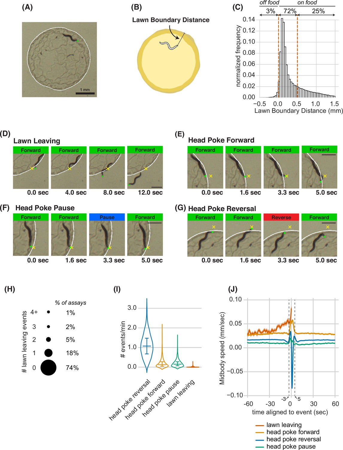
Animals make foraging decisions at the boundaries of bacterial food lawns.
(A) Image of C. elegans on a small lawn of bacteria. Head is indicated with a green dot, lawn boundary is indicated with a white line. Scale bar is 1 mm. (B) Schematic depicting lawn boundary distance measured as the distance from the head to the closest point on the lawn boundary. (C) Empirical distribution of lawn boundary distance in wild type datasets. Positive values indicate distances inside the lawn, negative values indicate distances outside the lawn. (D–G) Four example images from behavioral sequences generating different types of foraging decisions. Scale bar is 0.5 mm in all panels. Head is indicated with a green dot in all panels. In E-G, yellow X indicates the maximum displacement of the head outside the lawn during head pokes. (D) Lawn leaving occurs when an animal approaches lawn boundary and fully crosses through it to explore the bacteria-free agar outside the lawn. Yellow X indicates the position on the lawn boundary encountered by worm’s head before exiting the lawn. (E) Head Poke Forward occurs when animal continues forward movement on the lawn during and after poking its head outside the lawn. (F) Head Poke Pause occurs when animal pauses following head poke before resuming forward movement on the lawn. (G) Head Poke Reversal is generated by a reversal following head poke before resuming forward movement on the lawn. (H) Number of lawn leaving events per animal in 40-min assay. Bubble sizes are proportional to the percentage of animals that execute each number of lawn leaving events within a 40-min assay. (I) Frequency of different foraging decisions. (J) Midbody speed aligned to different foraging decision types. Wild type dataset (C,H,I,J): n=1586 animals. Violin plots in (I) show median and interquartile range. In all time-averages, dark line represents the mean and shaded region represents the standard error. See Figure 1—source data 1.
-
Figure 1—source data 1
Quantification of various lawn boundary interaction behaviors from experiments in Figure 1.
- https://cdn.elifesciences.org/articles/88657/elife-88657-fig1-data1-v1.xlsx
Figure 1—figure supplement 1
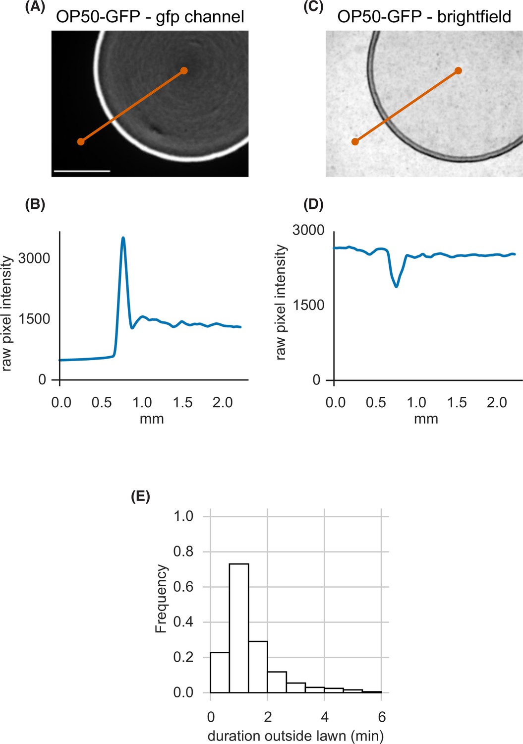
Small bacterial lawns are denser at the lawn boundary, and quantification of duration outside the lawn (A) A small lawn of bacteria expressing green fluorescent protein (GFP) imaged in the GFP channel.
White scale bar is 1 mm. (B) GFP intensity across the orange transect line plotted in (A) shows accumulation of bacterial cells near the lawn boundary in brighter GFP pixels. (C) An image of the same lawn in brightfield. (D) Brightfield intensity across the orange transect line plotted in (C) shows local darkening at the lawn boundary corresponding to bright GFP pixels in (A). (E) Duration of individual excursions outside the lawn. Quantified across wild type dataset (n=1586 animals). See Figure 1—source data 1.
Figure 1—video 1
Lawn boundary encounters lead to different behavioral responses: lawn leaving, head poke forward, head poke pause, and head poke reversal.
Green dot indicates the head position. White line indicates the lawn boundary. Forward and Reverse motion indicated in top left corner.
Figure 2 with 6 supplements
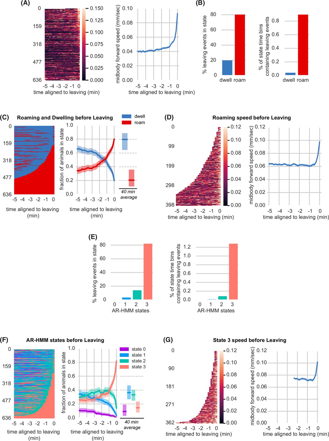
Lawn leaving is associated with high arousal states on multiple timescales.
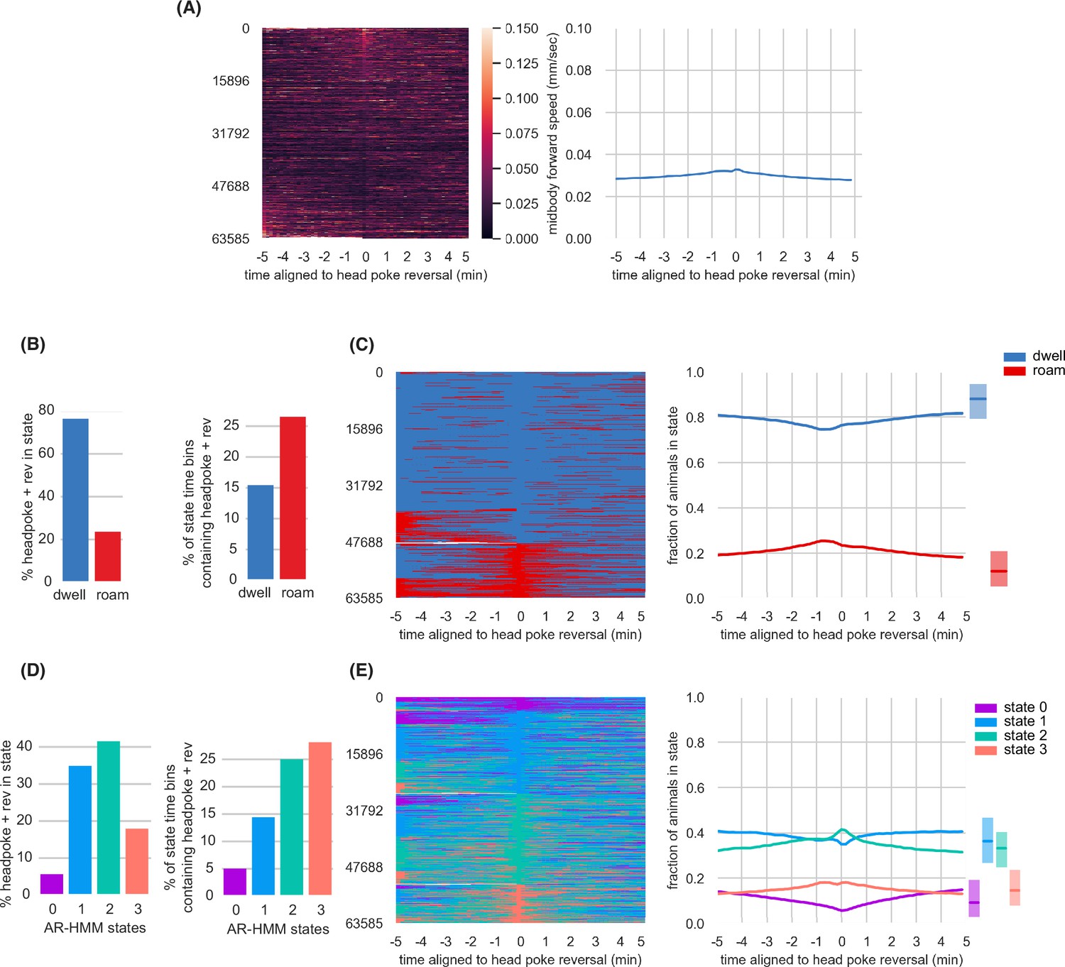
(A) Midbody forward speed aligned to lawn leaving. Left, heatmap of individual speed traces. Right, mean midbody forward speed computed across the heatmap traces. White space indicates missing data or times when animal was off the lawn. (B) Overlap of lawn leaving events with roaming and dwelling. Left, percentage of leaving events found in each state. Right, percentage of 10 s roaming or dwelling bins that contain a leaving event. (C) Roaming and dwelling aligned to lawn leaving. Left, heatmap of roaming/dwelling state classifications aligned to lawn leaving event. Center, fraction of animals in roaming or dwelling state prior to leaving. Right, total fraction of time spent roaming and dwelling in all assays that included a lawn-leaving event (n=371). Median is highlighted and interquartile range is indicated by shaded area. (D) Roaming speed aligned to lawn leaving. Left, heatmap showing speed of roaming animals before lawn leaving. Right, mean roaming speed computed at times when less than 10% of aligned traces had missing data. White space indicates times when animals were not roaming before leaving. (E) Overlap of lawn leaving events with AR-HMM states. Left, percentage of leaving events found in each state. Right, percentage of 10 s bins per AR-HMM state that contain a leaving event. (F) AR-HMM states aligned to lawn leaving. Left, heatmap of AR-HMM state classifications. Center, fraction of animals in each state prior to leaving. Right, total fraction of time spent in each AR-HMM state in all assays that included a lawn-leaving event (n=371). Median is highlighted and interquartile range is indicated by shaded area. (G) State 3 speed aligned to lawn leaving. Left, heatmap showing speed of animals in state 3 before lawn leaving. Right, mean state 3 speed computed at times when less than 10% of aligned traces had missing data. White space indicates times when animals were not in state 3 before leaving. See Figure 2—source data 1.
-
Figure 2—source data 1
Quantification of behavioral states surrounding lawn leaving events from experiments in Figure 2.
- https://cdn.elifesciences.org/articles/88657/elife-88657-fig2-data1-v1.xlsx
Figure 2—figure supplement 1
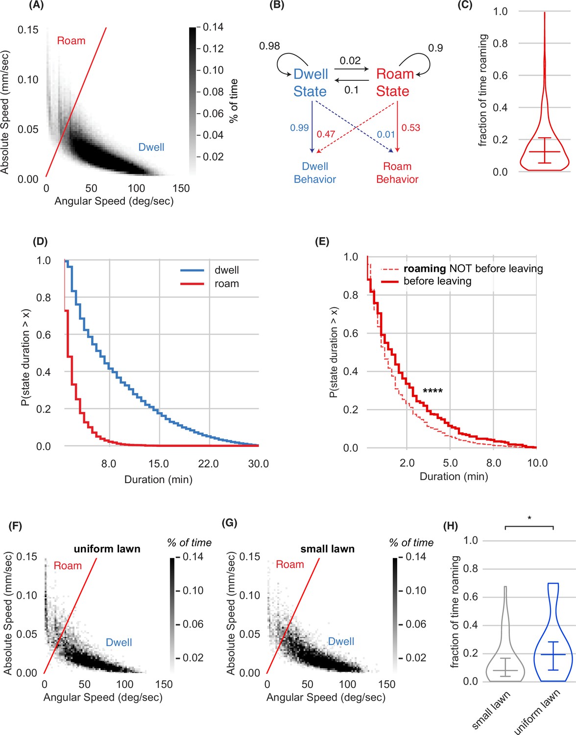
Roaming and dwelling states on small bacterial lawns.
(A) Scatter plot of average absolute speed and angular speed in 10 s intervals for wild type animals on small lawns (n=1586 animals, 380,640 bins). The boundary shown, used for all data in the paper, defines roaming (high speed/low angular speed) and dwelling (low speed/high angular speed). (B) Two-state Hidden Markov Model trained on wild-type animals. Roaming Behavior and Dwelling Behavior correspond to 10 s intervals either above or below the separating line in (A), respectively. Roaming and dwelling states are inferred from the Hidden Markov Model. Black arrows indicate transition probabilities between states and colored arrows represent emission probabilities. (C) Fraction of time spent roaming across wild type animals. (D) Complementary cumulative distribution functions (ccdfs) for roaming and dwelling state durations in minutes. (E) Empirical complementary cumulative distribution functions (ccdfs) comparing state durations of roaming states that did or did not precede a lawn leaving event. Statistics by Kolmogorov-Smirnov two-sample test. **** p<10–4. (F) Scatter plot of average absolute speed and angular speed in 10 s intervals for wild type animals on uniform lawns (n=31 animals, 7440 bins). (G) Same as (E) for animals on small lawns recorded in parallel with animals on uniform lawns (n=31 animals, 7440 bins). (H) Animals roam more on uniform lawns than on small lawns. * p<0.05 by Student’s t-test on logit-transformed data. Violin plots show median and interquartile range. See Figure 2—source data 1.
Figure 2—figure supplement 2
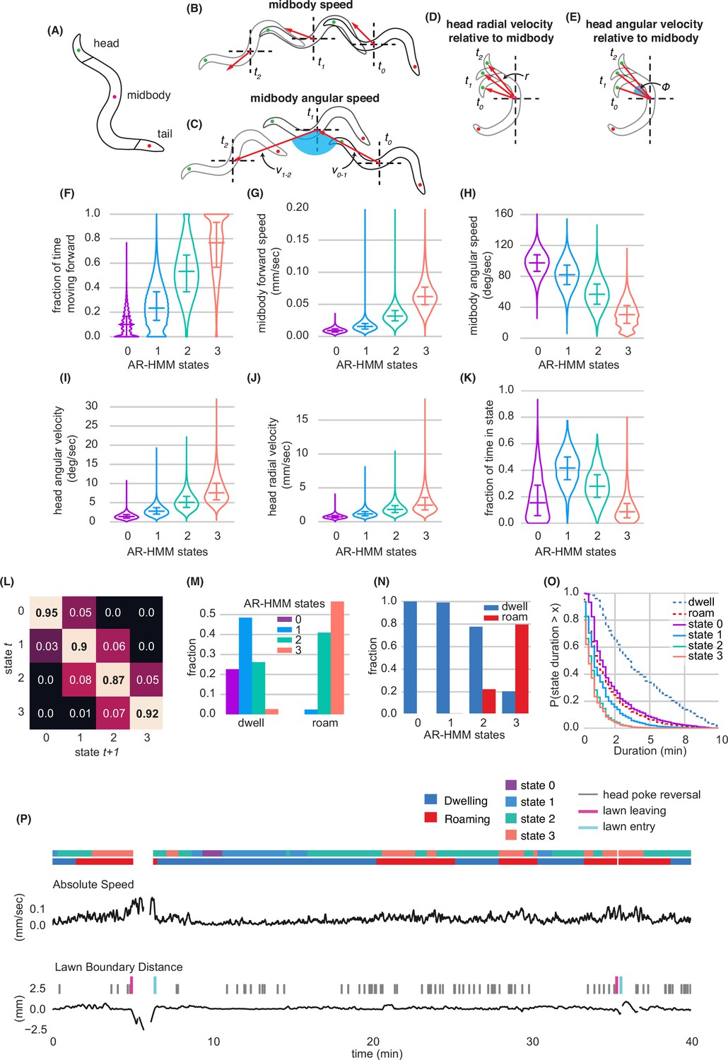
Modeling behavioral states across locomotory feature dimensions using an Autoregressive Hidden Markov Model.
(A) Schematic of animal body shape with key body points indicated. (B–E) Schematics illustrating derived behavioral features. See Methods for detailed description. (B) Midbody speed, (C) Midbody angular speed, (D) Head radial velocity relative to midbody, (E) Head angular velocity relative to midbody. (F–K) Quantification of behavioral parameters per animal while in each AR-HMM state. (F) Fraction of time spent moving forward, (G) Midbody forward speed, (H) Midbody angular speed, (I) Head angular velocity, (J) Head radial velocity, (K) Fraction of time spent in each state per animal. (L) Transition matrix for four-state AR-HMM. Rows index state at time t, columns index state at t+1. (M) Fraction of AR-HMM states found in roaming and dwelling states. (N) Fraction of roaming and dwelling states found in each AR-HMM state. (O) Empirical complementary cumulative distribution functions (ccdfs) comparing state durations from the 4-state AR-HMM to those of roaming and dwelling. (P) Example behavioral trace with two lawn leaving events. Absolute speed and lawn boundary distance are shown for a continuous 40-min assay. Foraging decisions are annotated with colored tick marks above lawn boundary distance trace. Roaming, Dwelling, and AR-HMM states are annotated above absolute speed with colored bars. Distributions are computed across wild type animals on small lawns (n=1586). Violin plots show median and interquartile range. See Figure 2—source data 1.
Figure 2—figure supplement 3
Head Poke Reversals are associated with small changes in arousal states.
(A) Midbody forward speed aligned to head poke reversals. Left, heatmap of individual speed traces. Right, mean midbody forward speed computed across the heatmap traces. (B) Overlap of head poke reversals with roaming and dwelling. Left, percentage of head poke reversals found in each state. Right, percentage of 10 s time bins roaming or dwelling that contain a head poke reversal. (C) Roaming and dwelling aligned to head poke reversals. Left, heatmap of roaming/dwelling state classifications aligned to head poke reversals. Center, fraction of animals in roaming or dwelling state prior to head poke reversals. Right, total fraction of time spent roaming and dwelling in all assays that included a head poke reversal. (D) Overlap of head poke reversals with AR-HMM states. Left, percentage of head poke reversals found in each state. Right, percentage of 10 s time bins per AR-HMM state that contain a head poke reversal. (E) AR-HMM states aligned to head poke reversals. Left, heatmap of roaming/dwelling state classifications aligned to head poke reversals. Center, fraction of animals in each AR-HMM state prior to head poke reversals. Right, total fraction of time spent in each AR-HMM state in all assays that included a head poke reversal. Data aligned to head poke reversals (n=63,585) from wild type animals (n=1586). Dark lines represent the mean and shaded region represents the standard error. In boxplots, median is highlighted, and interquartile range is indicated by shaded area. See Figure 2—source data 1.
Figure 2—figure supplement 4
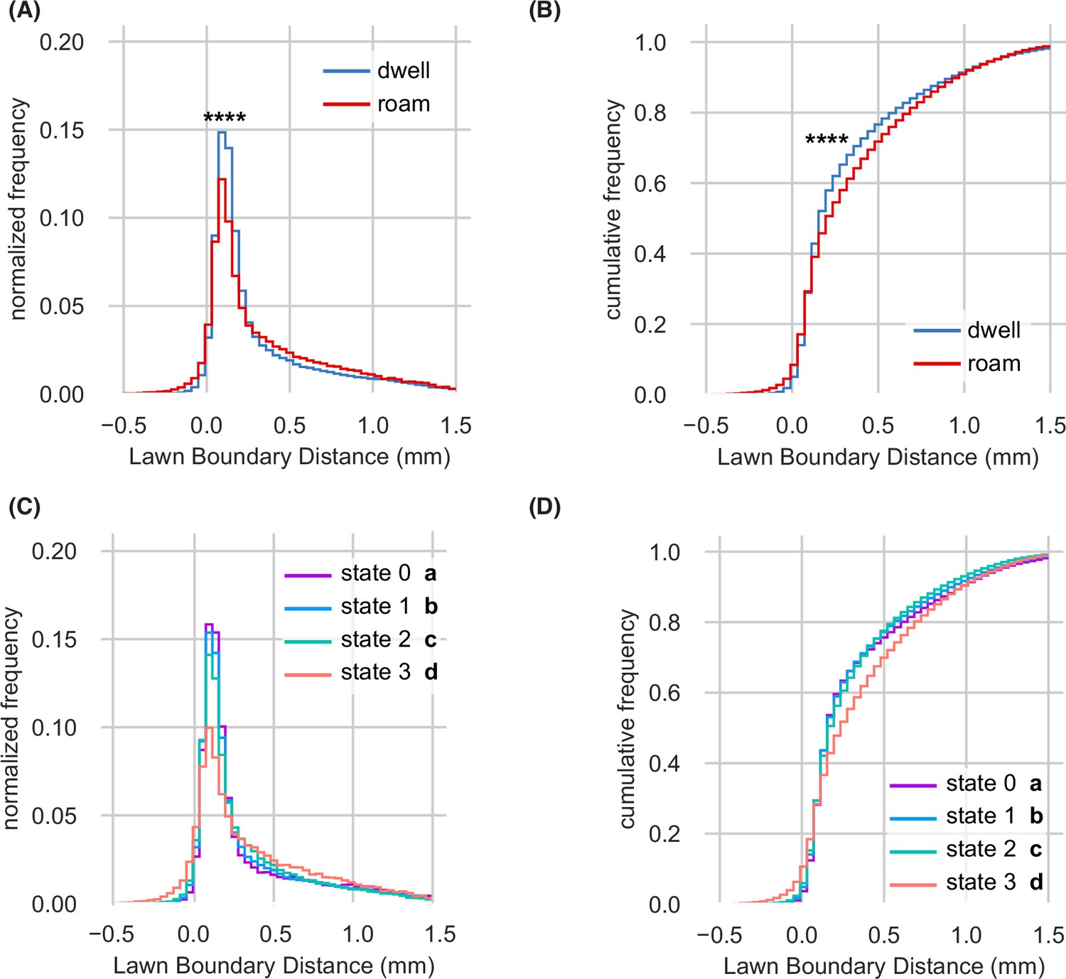
Lawn boundary distance distributions by HMM state (A–D) Empirical distributions of lawn boundary distance by HMM state.
Positive values indicate distances inside the lawn, negative values indicate distances outside the lawn (See Figure 1). (A) Lawn boundary distance of animals while roaming and dwelling. Statistics by Kolmogorov-Smirnov two-sample test. (B) Same as (A) but plotted as a cumulative distribution. (C) Lawn boundary distance of animals in each state of four-state AR-HMM. Statistics by Kolmogorov-Smirnov two-sample tests with Bonferroni correction. (D) Same as (C) but plotted as a cumulative distribution. Distributions are computed across wild type animals on small lawns (n=1586). In (A-B), **** p<10–4. In (C-D), each AR-HMM state is significantly different from all others (a-d), although effect sizes are small.
Figure 2—video 1
Example of animal behavior with roaming and dwelling annotated.
Animal shown corresponds to the behavior before and after the first lawn leaving event in Figure 2—figure supplement 2P.
Green dot indicates the head position. White line indicates the lawn boundary. Forward and Reverse motion indicated in top left corner. Speed indicated top middle. Time stamps indicated top right. Video sped up 7 x.
Figure 2—video 2
The same animal and time steps as in Figure 2—video 1, except annotated with AR-HMM states instead of roaming and dwelling.
Figure 3 with 1 supplement
Food intake regulates arousal states and lawn leaving.
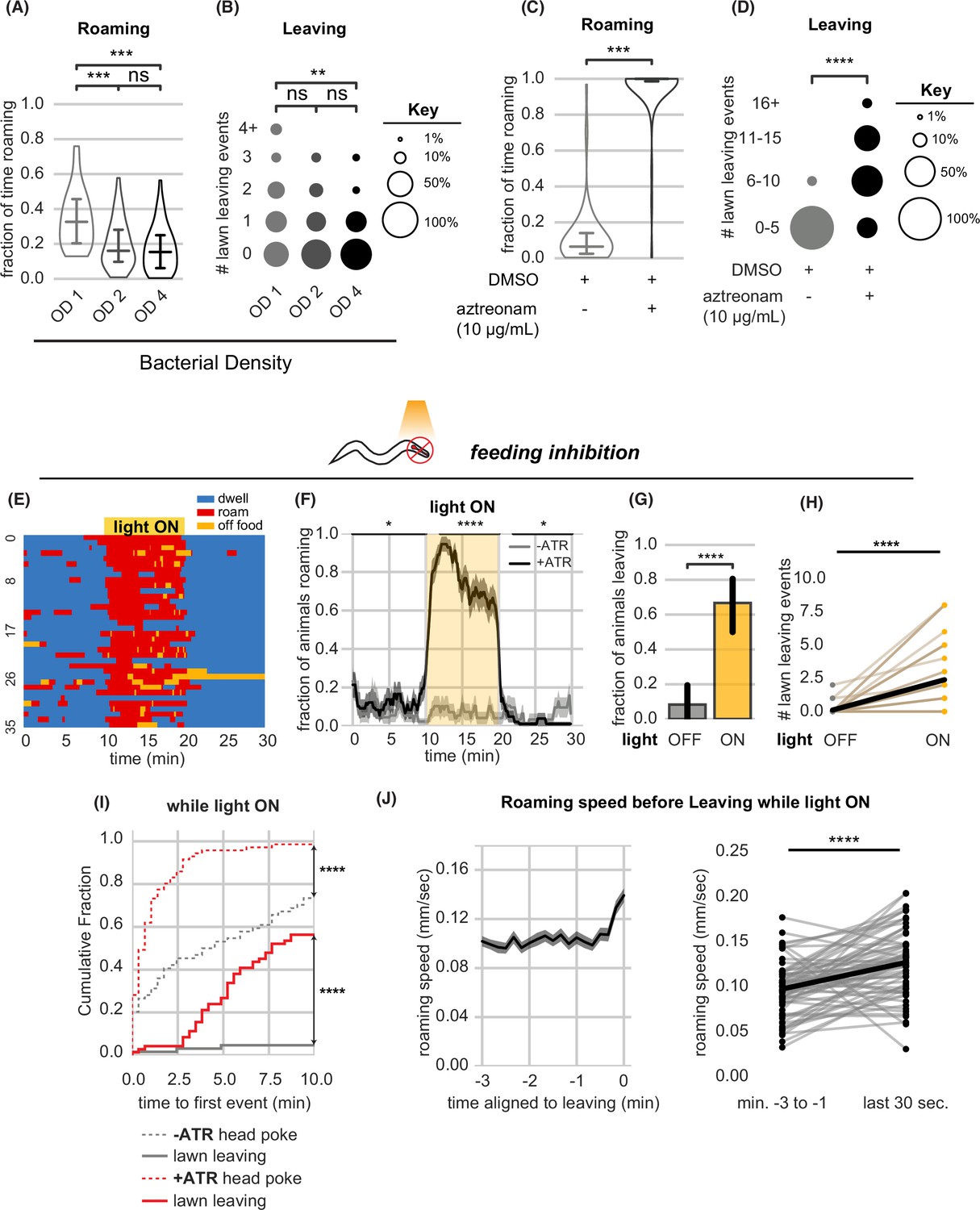
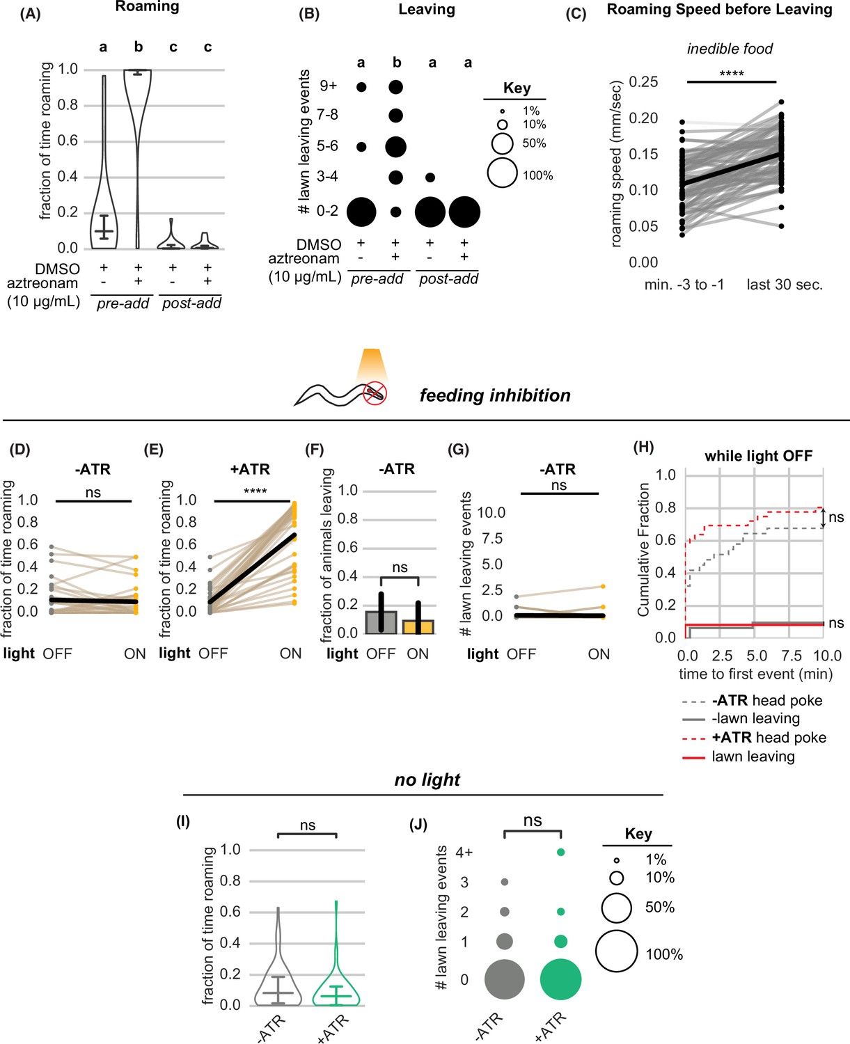
(A–B) Increasing bacterial density suppresses roaming and leaving. (A) Fraction of time roaming on small lawns seeded with bacteria of different optical density (OD). OD1: n=45, OD2: n=46, OD4: n=47, Statistics by one-way ANOVA with Tukey’s post-hoc test on logit-transformed data. (B) Number of lawn leaving events per animal in the same assays as (A). Statistics by Kruskal-Wallis test with Dunn’s multiple comparisons test. (C–D) Animals on inedible food roam and leave lawns more than animals on edible food. (C) Fraction of time roaming on inedible bacteria generated by adding aztreonam dissolved in DMSO to E. coli growing on plates.+DMSO/+aztreonam n=64,+DMSO (control) n=66, Statistics by Student’s t-test performed on logit-transformed data. (D) Number of lawn leaving events in the same assays as (C). Statistics by Mann-Whitney U-test. (E–J) Feeding inhibition by optogenetic depolarization of pharyngeal muscles stimulates roaming and lawn leaving. (E) Heatmap showing roaming and dwelling for animals before, during, and after 10 min optogenetic feeding inhibition. Data for animals pre-treated with all-trans retinal (+ATR) is shown. (F) Fraction of animals roaming before, during, and after optogenetic feeding inhibition. Light ON period denoted by yellow shading (+ATR n=36). Control animals not pre-treated with all-trans retinal (-ATR n=32). Statistics by Student’s t-test comparing +/-ATR data averaged and logit-transformed during intervals indicated by black lines above plots: Minutes 0–10, 12–20, 22–30. (G) A greater fraction of animals leave lawns during feeding inhibition. Statistics by Fisher’s exact test. (H) Number of lawn leaving events in the same assays as (G). Statistics by Wilcoxon rank-sum test. (I) Cumulative distribution of time until the first head poke reversal or lawn leaving event during feeding inhibition. Statistics by Kolmogorov-Smirnov two-sample test. (J) Roaming animals accelerate before leaving during feeding inhibition. Left, mean roaming speed of animals before leaving. Right, quantification of roaming speed increase from minutes –3 to –1 to the last 30 s before leaving. Statistics by Wilcoxon rank-sum test. Statistics: ns, not significant, * p<0.05, *** p<10–3,**** p<10–4 In time-averages (F,J), dark line represents the mean and shaded region represents the standard error. Violin plots show median and interquartile range. In (H), each dot pair connected by a line represents data from a single animal. In (J), each dot pair connected by a line represents data preceding a single lawn leaving event. Thick black line indicates the average. See Figure 3—source data 1.
-
Figure 3—source data 1
Quantification of roaming and lawn leaving from experiments in Figure 3.
- https://cdn.elifesciences.org/articles/88657/elife-88657-fig3-data1-v1.xlsx
Figure 3—figure supplement 1
Further quantification of roaming and leaving behaviors under food intake inhibition.
(A–B) Aztreonam affects roaming and leaving by affecting bacterial growth. In ‘pre-add’ conditions, the drug is added to liquid cultures and agar plates during bacterial growth. In ‘post-add’ conditions, the drug is added after bacterial growth just before testing behavior. (A) Fraction of time roaming. Different letters mark significant differences in roaming by logit-transformation followed by one-way ANOVA and Tukey’s post hoc test. (pre-add:+DMSO/+aztreonam n=12,+DMSO (control) n=15; post-add:+DMSO/+aztreonam n=12,+DMSO (control) n=16). (B) Number of lawn leaving events in the same assays as (A). Different letters mark significant differences in leaving by Kruskal-Wallis followed by Dunn’s multiple comparisons test. (C) Animals on inedible food accelerate before leaving the lawn. Statistics by Wilcoxon rank-sum test. (D–G) Quantification of controls relating to optogenetic feeding inhibition experiments. (D) Light exposure does not induce roaming in animals not pre-treated with all-trans retinal. Statistics by paired t-test on logit-transformed data. (E) Light exposure reliably induces roaming in animals pre-treated with all-trans retinal. Statistics by paired t-test on logit-transformed data. (F) Light exposure does not increase the fraction of animals that leave lawns when animals are not pre-treated with all-trans retinal. Statistics by Fisher’s exact test. (G) Light exposure does not increase the number of lawn leaving events when animals are not pre-treated with all-trans retinal. Statistics by Wilcoxon rank-sum test. (H) Cumulative distribution of time until the first head poke reversal or lawn leaving event while the light is OFF. Statistics by Kolmogorov-Smirnov two-sample test. (I–J) Quantification of roaming and leaving in animals with or without pre-treatment with all-trans retinal without light exposure. (-ATR n=67,+ATR n=57). (I) Pre-treatment with all-trans retinal does not alter the fraction of time roaming. Statistics by Student’s t-test on logit-transformed data. (J) Pre-treatment with all-trans retinal does not alter the number of lawn leaving events per animal. Statistics by Mann-Whitney U test. Statistics: ns not significant (p>0.05), **** p<10–4 Violin plots show median and interquartile range. In (D,E,G), each dot pair connected by a line represents data from a single animal. In (C), each dot pair connected by a line represents data preceding a single lawn leaving event. See Figure 3—source data 1.
Figure 4 with 1 supplement
Neuromodulatory signaling mutants retain coupling of arousal and leaving.
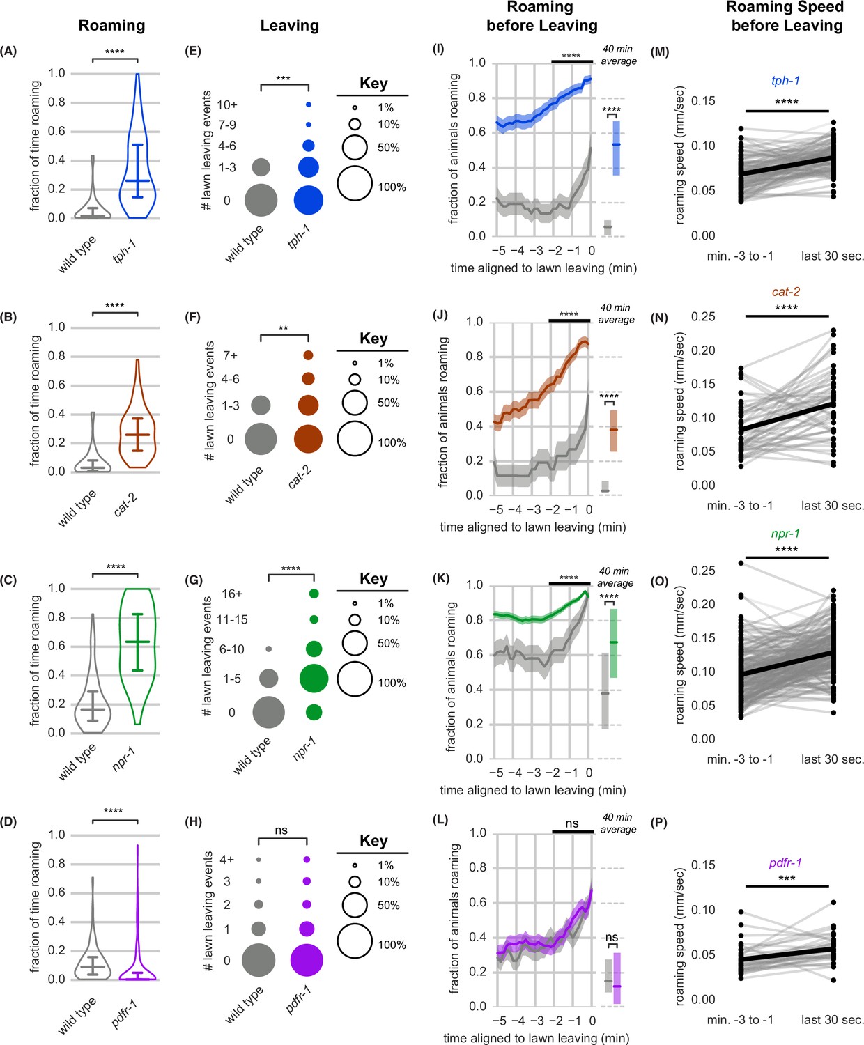
(A–P) Roaming, lawn leaving, roaming before leaving, and roaming speed quantified across mutants in four neuromodulatory genes known to alter roaming and dwelling: tph-1, cat-2, npr-1, and pdfr-1. (A–D) Fraction of time roaming. Statistics by Student’s t-test on logit-transformed data. (E–H) Number of lawn leaving events per animal. Statistics by Mann-Whitney U test. (I–L) Fraction of animals roaming before lawn leaving. Left, fraction of animals roaming in the last 5 min before lawn leaving. WT and mutant roaming fractions were compared over the two minutes prior to leaving (black bar). Right, total fraction of time spent roaming and dwelling in all assays that included a lawn-leaving event. Statistics by Student’s t-test on logit-transformed data. Note that roaming levels were unusually low (A,B,I,J) or high (C,K) in the wild-type controls for these groups, and therefore genotypes cannot be compared across different experimental panels. (M–P) Roaming speed before leaving computed at times when less than 10% of aligned traces had missing data. Paired plots indicate the average speed from minutes –3 to –1 and in the last 30 s before leaving per animal. Statistics by Wilcoxon rank-sum test. Statistics: ns not significant (p>0.05), ** p<0.01, *** p<10–3, **** p<10–4 Violin plots and box plots show median and interquartile range. In time-averages, dark line represents the mean and shaded region represents the standard error. In paired plots (M-P), each dot pair connected by a line represents data preceding a single lawn leaving event. Thick black line indicates the average. (tph-1 n=139, wild type controls n=127; cat-2 n=88, wild type controls n=76; npr-1 n=91, wild type controls n=90; pdfr-1 n=265, wild type controls n=247). See Figure 4—source data 1.
-
Figure 4—source data 1
Quantification of roaming and lawn leaving from experiments in Figure 4.
- https://cdn.elifesciences.org/articles/88657/elife-88657-fig4-data1-v1.xlsx
Figure 4—figure supplement 1
Optogenetic feeding inhibition stimulates roaming and leaving in neuromodulatory mutants.
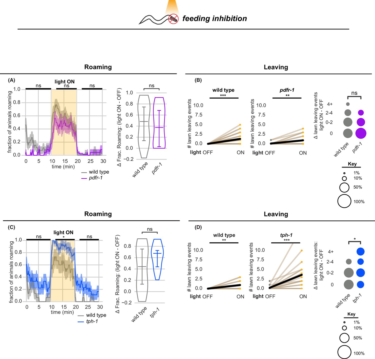
(A–B) Optogenetic feeding inhibition in pdfr-1 mutants. (A) Left, Fraction of animals roaming before, during and after optogenetic feeding inhibition in pdfr-1 mutants and paired wild type controls. Statistics by Student’s t-test comparing pdfr-1 and matched wild type data averaged and logit-transformed in intervals denoted by black bars above: Data compared at 0–10, 12–20, 22–30 min. Right, Difference in fraction of time roaming between light ON and light OFF conditions per animal. Statistics by Mann-Whitney U test. Left and Center, pdfr-1 animals and wild type controls execute more lawn leaving events under feeding inhibition while light is ON. Statistics by Wilcoxon rank-sum test. Right, difference in number of lawn leaving events between light ON and light OFF conditions per animal. Statistics by Mann-Whitney U test. (pdfr-1 n=23, wild type controls n=27). (C-D) Optogenetic feeding inhibition in tph-1 mutants. Same as (A) for tph-1 animals and matched controls. Same as (B) for tph-1 animals and matched controls. (tph-1 n=18, wild type controls n=16)Statistics: ns not significant (p>0.05), * p<0.05, ** p<0.01, *** p<10–3. Violin plots show median and interquartile range. In time-averages, dark line represents the mean and shaded region represents the standard error. In paired plots, each dot pair connected by a line represents data from a single animal. Thick black line indicates the average. See Figure 4—source data 1.
Figure 5 with 3 supplements
Acute circuit manipulation drives deterministic roaming and probabilistic leaving.
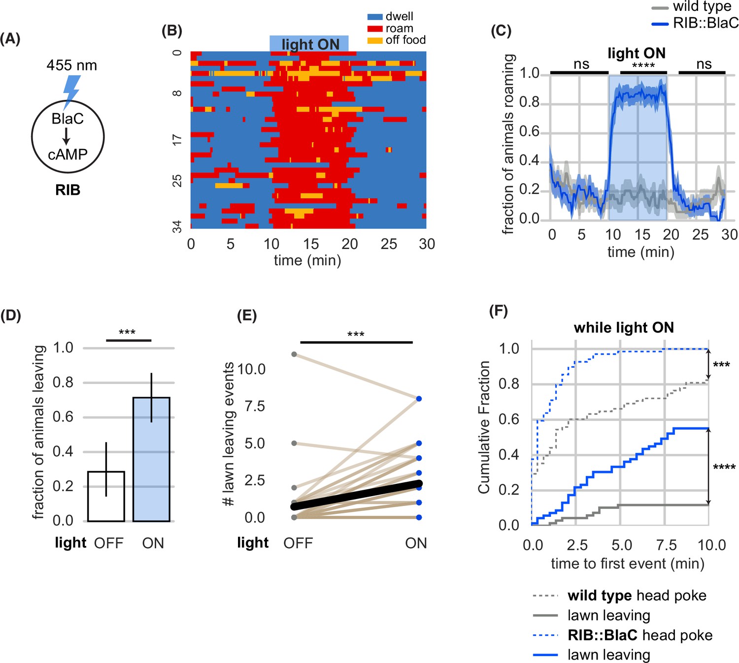
(A) Experimental design. Stimulation of bacterial light-activated adenylyl cyclase (BlaC) with 455 nm light increases cAMP synthesis in RIB::BlaC neurons. (B) Heatmap showing roaming and dwelling for RIB::BlaC animals before, during, and after 10-min optogenetic stimulation. (C) Fraction of animals roaming before, during, and after optogenetic blue light stimulation. Light ON period denoted by blue shading. Control animals are wild type. Statistics by Student’s t-test comparing RIB::BlaC and wild-type animals averaged and logit-transformed during intervals indicated by black lines above plots: Data compared at 0–10, 12–20, 22–30 min. (D) A greater fraction of RIB::BlaC animals leave lawns when the light is ON vs. OFF. Statistics by Fisher’s exact test. (E) Number of lawn leaving events under the same conditions as (D). Statistics by Wilcoxon rank-sum test. (F) Cumulative distribution of time until the first head poke reversal or lawn leaving event while the light is ON. Statistics by Kolmogorov-Smirnov two-sample test. Statistics: ns not significant (p>0.05), ** p<0.01, *** p<10–3, **** p<10–4 In time-averages (C), dark line represents the mean and shaded region represents the standard error. (RIB::BlaC n=35, wild type n=34) In (E), each dot pair connected by a line represents data from a single animal. Thick black line indicates the average. See Figure 5—source data 1.
-
Figure 5—source data 1
Quantification of roaming and lawn leaving from experiments in Figure 5.
- https://cdn.elifesciences.org/articles/88657/elife-88657-fig5-data1-v1.xlsx
Figure 5—figure supplement 1
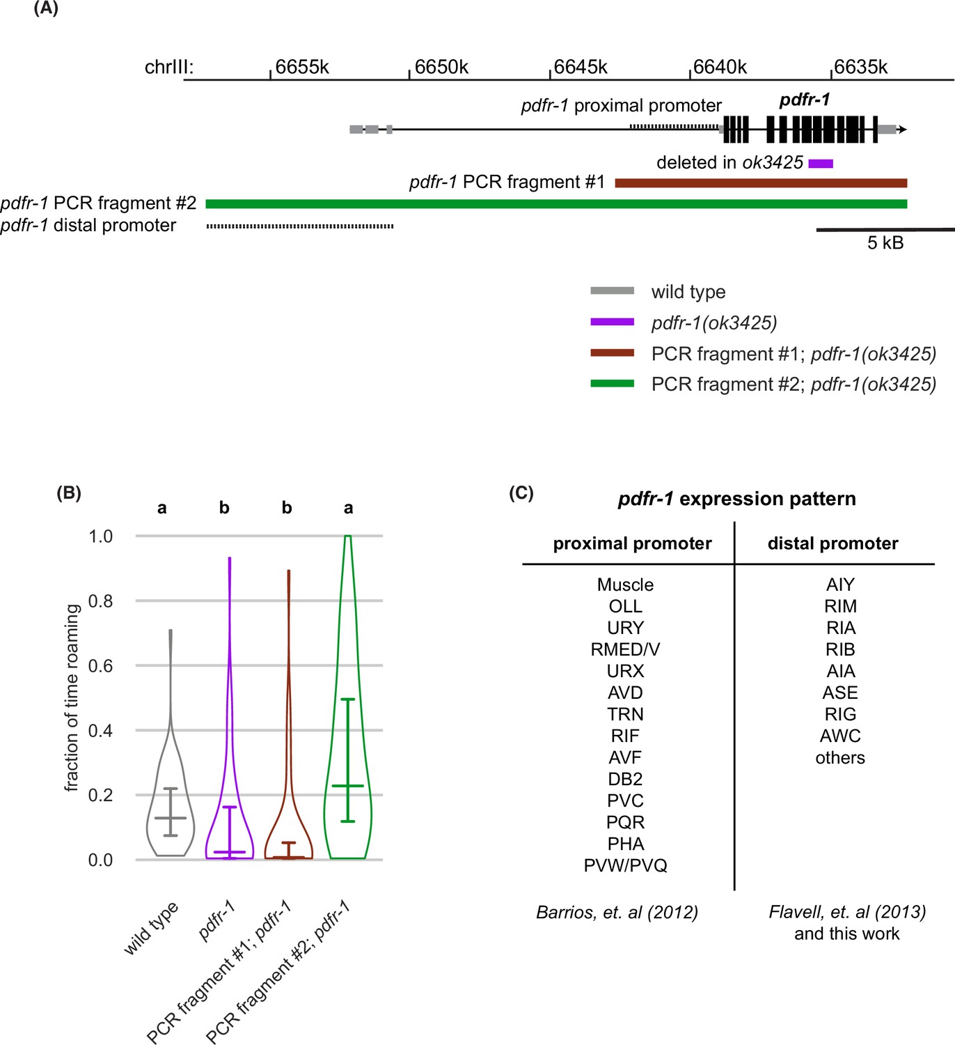
pdfr-1 genomic characteristics and expression patterns.
(A) Genomic region surrounding pdfr-1 (black boxes represent coding exons, gray boxes are non-coding exons), region deleted in pdfr-1(ok3425) mutants, proximal and distal promoters, PCR fragments used in transgenic rescue experiments. (B) Rescue of pdfr-1 roaming phenotype by transgenic expression from the PCR fragments illustrated in (A). Different letters mark significant differences in roaming by logit-transformation followed by Tukey’s post hoc test (wild type n=55, pdfr-1 n=59, PCR fragment #1; pdfr-1 n=46, PCR fragment #2; pdfr-1 n=51). Violin plots show median and interquartile range. (C) pdfr-1 expression patterns from the proximal and distal promoters as reported (Barrios et al., 2012, Flavell et al., 2013) and from this work. See Figure 5—source data 1.
Figure 5—figure supplement 2
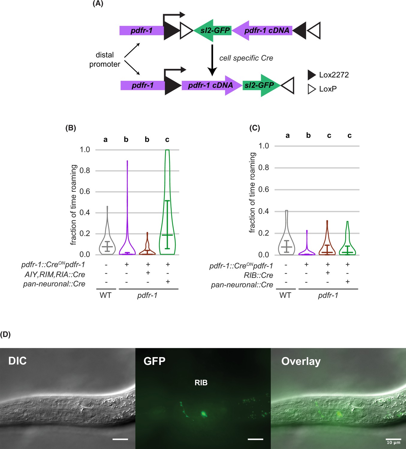
Transgenic rescue of pdfr-1 in RIB neurons restores roaming (A) Schematic depicting intersectional cell-specific rescue of pdfr-1 using an inverted Cre-Lox strategy.
(B) Restoring pdfr-1 expression in AIY, RIM, and RIA neurons did not rescue roaming on small lawns (wild type n=64, inverted pdfr-1 transgene n=64, AIY, RIM, RIA pdfr-1 rescue n=64, pan-neuronal::Cre rescue n=67). (C) Restoring pdfr-1 expression in RIB neurons rescued roaming comparably to pan-neuronal rescue on small lawns (wild type n=27, inverted pdfr-1 transgene n=32, RIB pdfr-1 rescue n=33, pan-neuronal::Cre rescue n=31). (D) Differential interference contrast (DIC), GFP fluorescence and composite images of an animal expressing pdfr-1 in the RIB neurons using the transgenic strategy shown in (A). Scale bar is 10 μm. Statistics: In (B-C), different letters mark significant differences in roaming by logit-transformation followed by Tukey’s post hoc test. Violin plots (B,C) show median and interquartile range. See Figure 5—source data 1.
Figure 5—figure supplement 3
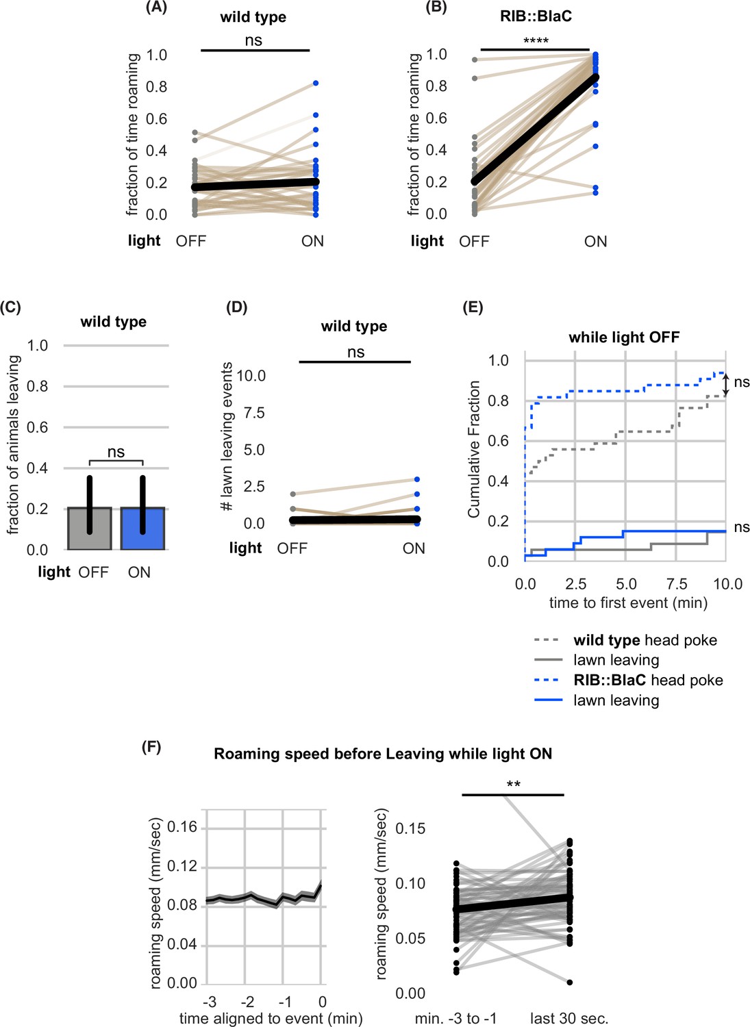
Further quantification and controls of RIB::BlaC experiments.
(A–E) Quantification of RIB::BlaC controls. (A) Blue light stimulation does not induce roaming in wild-type animals. Statistics by paired t-test on logit-transformed data. (B) Blue light stimulation reliably induces roaming in RIB::BlaC animals. Statistics by paired t-test on logit-transformed data. (C) Blue light stimulation does not elevate the fraction of wild-type animals that leave lawns. Statistics by Fisher’s exact test. (D) Blue light stimulation does not elevate the number of lawn leaving events per wild type animal. Statistics by Wilcoxon rank-sum test. (E) Cumulative distribution of time until the first head poke reversal or lawn leaving event while the light is OFF. Statistics by Kolmogorov-Smirnov two-sample test. (F) Roaming animals only accelerate slightly before leaving during RIB BlaC stimulation. Left, mean roaming speed of animals before leaving. Right, quantification of roaming speed changes before leaving. Statistics by Wilcoxon rank-sum test. (RIB BlaC n=35, wild type n=34). Statistics: ns not significant (p>0.05), **** p<10–4 In paired plots (A,B,D), each dot pair connected by a line represents data from a single animal. Thick black line indicates the average. See Figure 5—source data 1.
Figure 6 with 4 supplements
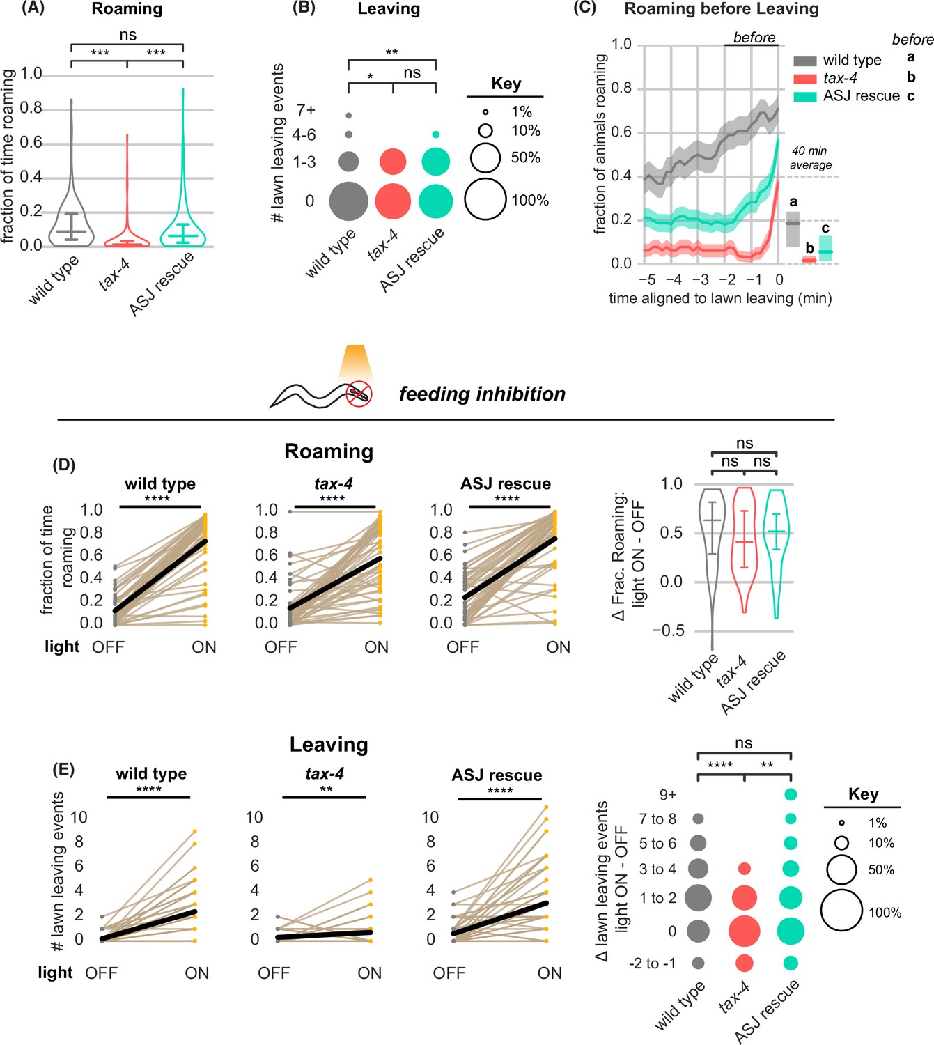
tax-4-expressing sensory neurons couple roaming and lawn leaving.
(A–C) Roaming and leaving in tax-4 mutants, and rescue by tax-4 expression in ASJ neurons (wild type n=143, tax-4 n=156, tax-4 ASJ rescue n=148). Additional features of roaming and leaving are shown in Figure 6—figure supplement 1; results with additional rescued neurons are in Figure 6—figure supplement 2. (A) Fraction of time roaming. Statistical tests, one-way ANOVA followed by Tukey’s post hoc test on logit-transformed data. (B) Number of lawn-leaving events per animal. Statistical tests, Kruskal-Wallis followed by Dunn’s multiple comparisons test. (C) Fraction of animals roaming before lawn-leaving. Left, fraction of animals roaming in the last 5 min before lawn leaving. Roaming fractions were compared over the 2 min prior to leaving (black bar). Right, total fraction of time spent roaming and dwelling in all assays that included a lawn-leaving event. Key, statistical tests of differences in roaming two minutes before leaving by one-way ANOVA followed by Tukey’s post hoc test on logit-transformed data. (D–E) Optogenetic feeding inhibition in tax-4 mutants and rescued strains (wild type n=70, tax-4 n=66, tax-4 ASJ rescue n=68). (D) Left, Fraction of time spent roaming under optogenetic feeding inhibition in tax-4 and ASJ rescue strain. Statistics by paired t-test on logit-transformed data. Right, Difference in the fraction of time roaming when the light is ON and OFF. Statistics by one-way ANOVA followed by Tukey’s post hoc test on logit-transformed data. (E) Left, Number of lawn leaving events under optogenetic feeding inhibition in tax-4 and ASJ rescue strain. Statistics by Wilcoxon rank-sum test. Right, Difference in the number of lawn leaving events when the light is ON and OFF. Statistics by Kruskal-Wallis test followed by Dunn’s multiple comparisons test. ns not significant (p>0.05), * p<0.05, *** p<10–3, **** p<10–4 Violin plots and box plots (A,D) show median and interquartile range. In time-averages (C), dark line represents the mean and shaded region represents the standard error. In paired plots (D,E), each dot pair connected by a line represents data from a single animal. Thick black line indicates the average. See Figure 6—source data 1.
-
Figure 6—source data 1
Quantification of roaming and lawn leaving from experiments in Figure 6.
- https://cdn.elifesciences.org/articles/88657/elife-88657-fig6-data1-v1.xlsx
Figure 6—figure supplement 1
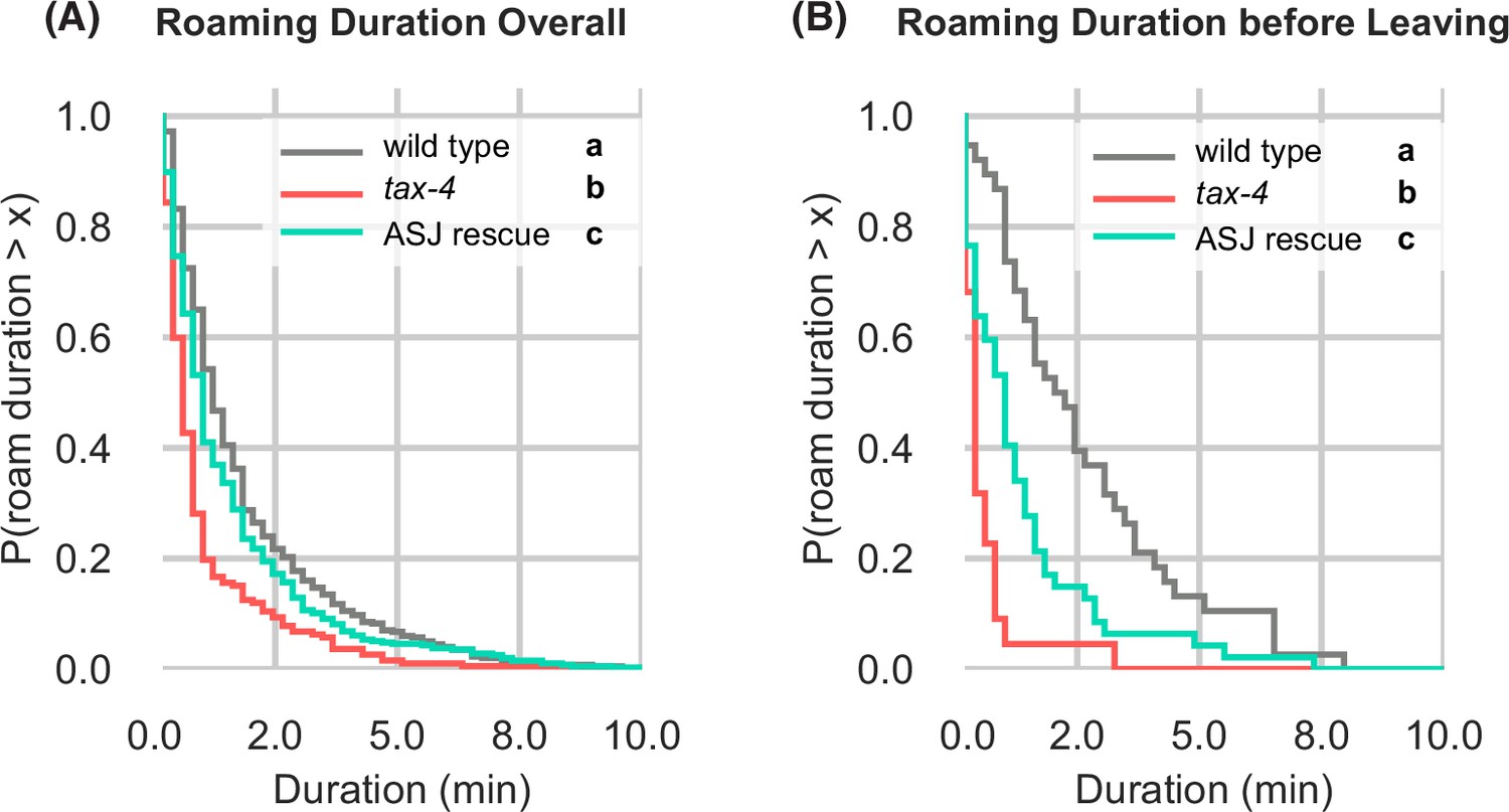
Further quantification of tax-4 mutants and tax-4 ASJ rescue on edible food (A) Complementary cumulative distribution functions (ccdfs) for overall roam state durations for wild type, tax-4, and tax-4 rescued in ASJ.
Different letters mark significant differences by Kolmogorov-Smirnov two-sample tests with Bonferroni correction. (B) Same as (A) for roam state durations before leaving events. Wild type n=143, tax-4 n=156, tax-4 ASJ rescue n=148. Statistics: different letters indicate significant differences. See Figure 6—source data 1.
Figure 6—figure supplement 2
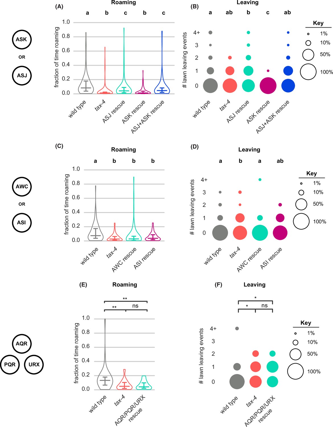
tax-4 rescue in additional tax-4-expressing neurons (A–B) Quantification of roaming and leaving in tax-4 mutants with tax-4 rescued in ASJ, ASK or ASJ +ASK neurons (wild type n=95, tax-4 n=104, ASJ rescue n=91, ASK rescue n=101, ASJ +ASK rescue n=105).
(A) ASJ or ASJ +ASK tax-4 rescue restores roaming to tax-4 mutants. (B) ASK tax-4 rescue suppresses lawn leaving below tax-4 levels. (C–D) Quantification of roaming and leaving in tax-4 mutants with tax-4 rescued in AWC or ASI neurons (wild type n=79, tax-4 n=88, AWC rescue n=68, ASI rescue n=77). (C) AWC or ASI tax-4 rescue fails to restore roaming to tax-4 mutants. (D) AWC tax-4 rescue restores lawn leaving to wild-type levels. (E–F) Quantification of roaming and leaving in tax-4 mutants with tax-4 rescued in AQR/PQR/URX neurons (wild type n=35, tax-4 n=32, AQR/PQR/URX rescue n=19). (E) AQR/PQR/URX tax-4 rescue fails to restore roaming to tax-4 mutants. (F) AQR/PQR/URX tax-4 rescue fails to restore lawn leaving. Violin plots (A,C,E) show median and interquartile range. Statistics: Different letters mark significant differences. ns not significant (p>0.05), * p<0.05, ** p<0.01, *** p<10–3. Statistical tests for differences in fraction of time roaming by one-way ANOVA followed by Tukey’s post hoc test on logit-transformed data. Statistical tests for differences in lawn leaving by Kruskal-Wallis test followed by Dunn’s multiple comparisons test. See Figure 6—source data 1.
Figure 6—figure supplement 3
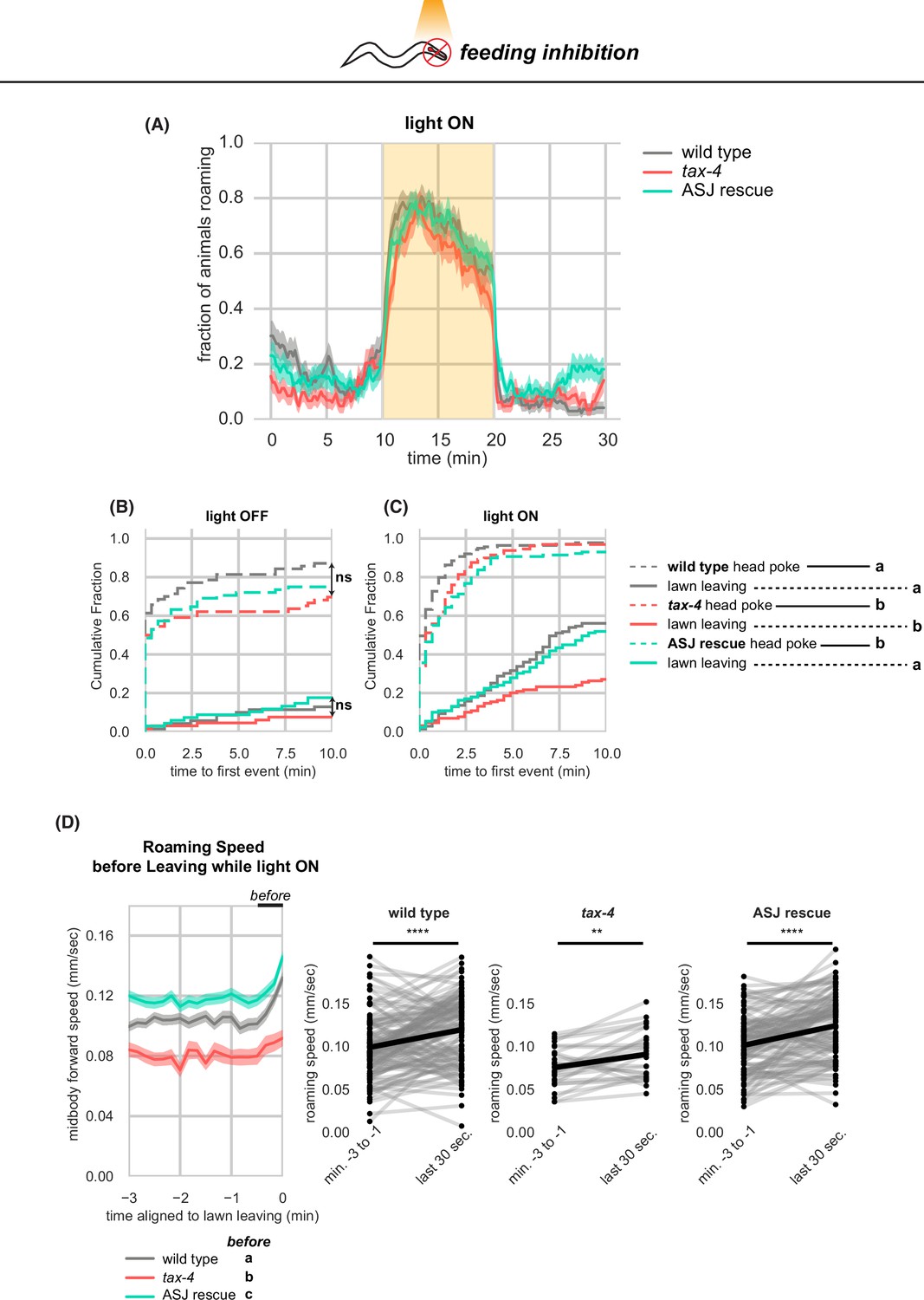
Further quantification of tax-4 mutants and tax-4 rescue upon optogenetic feeding inhibition (A-D) Effects of tax-4 on roaming and leaving behavior induced by optogenetic feeding inhibition.
(A) Fraction of animals roaming before, during, and after optogenetic feeding inhibition. Light ON period denoted by yellow shading. (B) Cumulative distribution of time until the first head poke reversal or lawn leaving event while the light is OFF. Statistics by all pairwise Kolmogorov-Smirnov two-sample tests, Bonferroni corrected. (C) Same as (D) for when the light is ON. Pairwise significant differences in time to first lawn leaving are indicated in the figure legend. (D) Left, Roaming speed before leaving while the light is ON computed at times when less than 10% of aligned traces had missing data. Roaming speed from the last 30 s is averaged and compared by statistical testing: significant differences are reported in the figure legend under ‘before’. Right, paired plots indicate the average speed from minutes –3 to –1 and in the last 30 s before leaving per animal. Each dot pair connected by a line represents data preceding a single lawn leaving event. Thick black line indicates the average. Statistics: ** p<0.01, *** p<10–3, Different letters mark significant differences. Violin plots (B,C) show median and interquartile range. See Figure 6—source data 1.
Figure 6—figure supplement 4
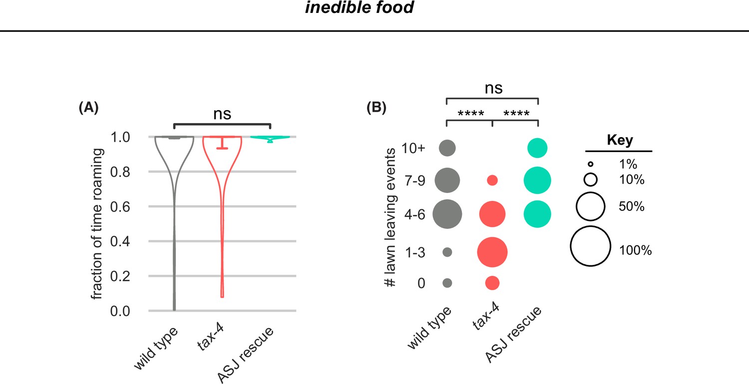
tax-4 mutants leave less on inedible food and ASJ rescue restores leaving.
(A–B) In these panels, wild type n=30, tax-4 n=22, tax-4 ASJ rescue n=10 on inedible food generated by pre-treatment of bacterial lawns with aztreonam before growth. (A) Wild type, tax-4 and tax-4 ASJ rescue animals all roam near-constantly on inedible food. Statistical tests of differences in roaming by one-way ANOVA followed by Tukey’s post hoc test on logit-transformed data. (B) tax-4 mutants leave lawns of inedible bacteria less frequently than wild type. tax-4 ASJ rescue restores lawn leaving. Statistical tests of differences in lawn leaving by Kruskal-Wallis followed by Dunn’s multiple comparisons test. See Figure 6—source data 1.
Tables
Key resources table
| Reagent type (species) or resource | Designation | Source or reference | Identifiers | Additional information |
|---|---|---|---|---|
| Strain, strain background (Caenorhabditis elegans, N2 hermaphrodite) | Wild type | Yoshimura et al., 2019 | PD1074 (now CGC1) | Used in all figures except Figure 4 tph-1 and cat-2 controls |
| Strain, strain background (Caenorhabditis elegans, N2 hermaphrodite) | Wild type | This paper | ID_BargmannDatabase:CX0001 | Used as wild type controls in Figure 4 tph-1 and cat-2 experiments |
| Strain, strain background (Caenorhabditis elegans, N2 hermaphrodite) | pharynx ReaChR | This paper | ID_BargmannDatabase:CX16279 | Figures 3 and 6 and supplements |
| Strain, strain background (Caenorhabditis elegans, N2 hermaphrodite) | pdfr-1 | Flavell et al., 2013 | ID_BargmannDatabase:CX14295 | Figure 4 |
| Strain, strain background (Caenorhabditis elegans, N2 hermaphrodite) | tph-1 | https://cgc.umn.edu/strain/MT15434 | ID_BargmannDatabase:MT15434 | Figure 4 |
| Strain, strain background (Caenorhabditis elegans, N2 hermaphrodite) | cat-2 | Stern et al., 2017 | ID_BargmannDatabase:CX11078 | Figure 4 |
| Strain, strain background (Caenorhabditis elegans, N2 hermaphrodite) | npr-1 | Jang et al., 2017 | ID_BargmannDatabase:CX13663 | Figure 4 |
| Strain, strain background (Caenorhabditis elegans, N2 hermaphrodite) | pharynx ReaChR; pdfr-1 | This paper | ID_BargmannDatabase:CX16528 | Figure 4—figure supplement 1 |
| Strain, strain background (Caenorhabditis elegans, N2 hermaphrodite) | pharynx ReaChR; tph-1 | This paper | ID_BargmannDatabase:CX16529 | Figure 4—figure supplement 1 |
| Strain, strain background (Caenorhabditis elegans, N2 hermaphrodite) | RIB::BlaC | This paper | ID_BargmannDatabase:CX18471 | Figure 5, Figure 5—figure supplement 3 |
| strain, strain background (Caenorhabditis elegans, N2 hermaphrodite) | PCR fragment #1; pdfr-1 | Flavell et al., 2013 | ID_BargmannDatabase:CX14378 | Figure 5—figure supplement 1 |
| Strain, strain background (Caenorhabditis elegans, N2 hermaphrodite) | PCR fragment #2; pdfr-1 | Flavell et al., 2013 | ID_BargmannDatabase:CX14383 | Figure 5—figure supplement 1 |
| Strain, strain background (Caenorhabditis elegans, N2 hermaphrodite) | pdfr-1:: CreONpdfr-1 | Flavell et al., 2013 | ID_BargmannDatabase:CX14485 | Figure 5—figure supplement 2 |
| Strain, strain background (Caenorhabditis elegans, N2 hermaphrodite) | RIB pdfr-1 rescue; pdfr-1 | This paper | ID_BargmannDatabase:CX18302 | Figure 5—figure supplement 2 |
| Strain, strain background (Caenorhabditis elegans, N2 hermaphrodite) | pan-neuronal pdfr-1 rescue; pdfr-1 | Flavell et al., 2013 | ID_BargmannDatabase:CX14488 | Figure 5—figure supplement 2 |
| Strain, strain background (Caenorhabditis elegans, N2 hermaphrodite) | AIY, RIM, RIA pdfr-1 rescue; pdfr-1 | Flavell et al., 2013 | ID_BargmannDatabase:CX14271 | Figure 5—figure supplement 2 |
| Strain, strain background (Caenorhabditis elegans, N2 hermaphrodite) | tax-4 | Worthy et al., 2018 | ID_BargmannDatabase:CX13078 | Figure 6, Figure 6—figure supplements 1 and 2, 4 |
| Strain, strain background (Caenorhabditis elegans, N2 hermaphrodite) | ASJ rescue; tax-4 | This paper | ID_BargmannDatabase:CX11118 | Figure 6, Figure 6—figure supplements 2 and 4 |
| Strain, strain background (Caenorhabditis elegans, N2 hermaphrodite) | ASK rescue; tax-4 | This paper | ID_BargmannDatabase:CX13361 | Figure 6—figure supplement 2 |
| Strain, strain background (Caenorhabditis elegans, N2 hermaphrodite) | ASJ +ASK rescue; tax-4 | This paper | ID_BargmannDatabase:CX11110 | Figure 6—figure supplement 2 |
| Strain, strain background (Caenorhabditis elegans, N2 hermaphrodite) | AWC rescue; tax-4 | Worthy et al., 2018 | ID_BargmannDatabase:CX13790 | Figure 6—figure supplement 2 |
| Strain, strain background (Caenorhabditis elegans, N2 hermaphrodite) | ASI rescue; tax-4 | This paper | ID_BargmannDatabase:CX11558 | Figure 6—figure supplement 2 |
| Strain, strain background (Caenorhabditis elegans, N2 hermaphrodite) | URX/AQR/PQR rescue; tax-4 | This paper | ID_BargmannDatabase:CX11113 | Figure 6—figure supplement 2 |
| Strain, strain background (Caenorhabditis elegans, N2 hermaphrodite) | pharynx ReaChR; tax-4 | This paper | ID_BargmannDatabase:CX18452 | Figure 6, Figure 6—figure supplement 3 |
| Strain, strain background (Caenorhabditis elegans, N2 hermaphrodite) | pharynx ReaChR; tax-4; ASJ rescue | This paper | ID_BargmannDatabase:CX18538 | Figure 6, Figure 6—figure supplement 3 |
| Strain, strain background (Escherichia coli, OP50) | OP50 | Caenorhabditis Genetics Center (CGC) | https://cgc.umn.edu/strain/OP50 | |
| Chemical compound, drug | Aztreonam | Sigma | PZ0038 | CAS: 78110-38-0 |
| Chemical compound, drug | all trans-Retinal (ATR) | Sigma | R2500 | CAS: 116-31-4 |
| Software, algorithm | ImageJ | ImageJ (https://imagej.nih.gov/) | RRID:SCR_003070 | Version 1.50i |
| Software, algorithm | MATLAB | Mathworks (https://www.mathworks.com/) | RRID:SCR_001622 | Version R2018a, R2020a, R2021a, R2023a |
| Software, algorithm | FlyCapture | Pointgrey (https://www.ptgrey.com/) | Version FlyCap2 | |
| Software, algorithm | Python | Python (python.org) | RRID:SCR_008394 | Version 3.8.3 |
| Software, algorithm | tracking and analysis code | this paper; Scheer and Bargmann, 2023 | https://github.com/BargmannLab/Scheer_Bargmann2023 |
Additional files
-
Supplementary file 1
Sensory neurons and endocrine systems implicated in roaming and leaving behavior.
- https://cdn.elifesciences.org/articles/88657/elife-88657-supp1-v1.xlsx
-
Supplementary file 2
Lawn Leaving Events Per minute Roaming/Dwelling.
- https://cdn.elifesciences.org/articles/88657/elife-88657-supp2-v1.xlsx
-
Supplementary file 3
Strains and Plasmids.
- https://cdn.elifesciences.org/articles/88657/elife-88657-supp3-v1.xlsx
-
Supplementary file 4
p-values and Statistical Tests.
- https://cdn.elifesciences.org/articles/88657/elife-88657-supp4-v1.xlsx
-
MDAR checklist
- https://cdn.elifesciences.org/articles/88657/elife-88657-mdarchecklist1-v1.pdf
Download links
A two-part list of links to download the article, or parts of the article, in various formats.
Downloads (link to download the article as PDF)
Open citations (links to open the citations from this article in various online reference manager services)
Cite this article (links to download the citations from this article in formats compatible with various reference manager tools)
Sensory neurons couple arousal and foraging decisions in Caenorhabditis elegans
eLife 12:RP88657.
https://doi.org/10.7554/eLife.88657.3


