Epistasis facilitates functional evolution in an ancient transcription factor
Figures
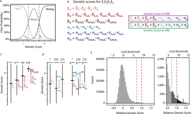
An ordinal regression model of the genetic architecture of transcription factor specificity.
(A) The ordinal logistic model. The probability that a protein variant is in each binding class is a logistic function of its genetic score. Thresholds between classes (dotted lines) correspond to scores at which the probability of being in two classes is equal. (B) A variant’s genetic score is the sum of the effects of the sequence states and combinations it contains, including main (1°), pairwise (2°), and third-order (3°) effects. Each state and combination has a term for its effect on generic binding averaged over REs (β, red) and another for its effect on specificity (σ, blue) for ERE vs. SRE; specificity terms are added or subtracted to give the genetic score on SRE or ERE, respectively. All terms are defined relative to the global average over all variants (β°). Components of the score for variant EGKA is shown as an example. (C) Schematic of reference-free model terms. Each term represents the average deviation of sequences containing a state (or combination) from the sum of the variant’s terms at lower orders, including the global average. Vertical and horizontal lines show range and mean of genetic scores for variants containing the specified states; *, any of the 20 amino acid states. (D) Reference-free specificity effects. Binding effects (red) are defined the same as in C. The global specificity effect (σ0) is the deviation from the global average for all genotypes on ERE (purple) vs. SRE (green). First order specificity effects (σ1s) are additional deviations from this global effect between ERE and SRE for genotypes with a particular amino acid at a particular site. (E) Distribution of genetic scores after fitting to the experimental DMS data for all 320,000 protein:DNA combinations. Scores were rescaled so that the global average is zero and the threshold score to be classified as a strong binder is 1. Dashed lines, interclass thresholds. Inset, right tail of the distribution. Estimated −ΔΔG values of binding associated with each genetic score are shown along the top, based on calibration to experimental binding data for a subset of variants. Arrows, biological reference sequences GSKV (SRE binder, green) and EGKA (ERE binder, purple).
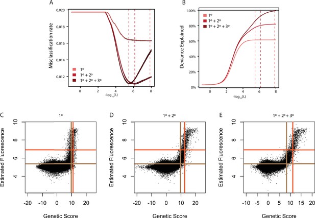
Model fitting and cross-validation.
(A) Average misclassification rate. Misclassification rate was measured by 10-fold cross-validation. The x-axis gives the lambda value used in ridge regression for the models containing main effects (1°, light red), main and pairwise epistatic effects (1°+2°, medium red), and main, pairwise, and third-order epistatic effects (1°+2°+3°, Full model, dark red). In each case, variance around the estimate from 10 independent cross-validation runs is shown in black. Dashed lines show the lambda value at which misclassification error is minimized. (B) Deviance explained by each model as the lambda ridge regression penalty parameter is reduced. Deviance is measured as two times the difference in log(Likelihood) of the model compared to a saturated model that contains a single parameter for every data point and is thus a perfect predictor of genotype binding class. For generalized linear models, deviance is the measure analogous to R2. Dashed lines are the same as in A and thus maximize deviance explained without over-fitting. (C) Comparison of estimated genetic score and mean fluorescence for the main effects only model (1°). Threshold genetic score between Null and Weak genotypes (vertical brown line) and between Weak and Strong genotypes (vertical orange line) are shown. The dashed horizontal lines show the 10th percentile of variants estimated as weak (orange) or strong (brown) based on their mean fluorescence. (D) Same as C, but for the model containing pairwise epistasis (1°+2°). (E) Same as C, but for the full model containing pairwise and third order epistasis (1°+2°+3°).
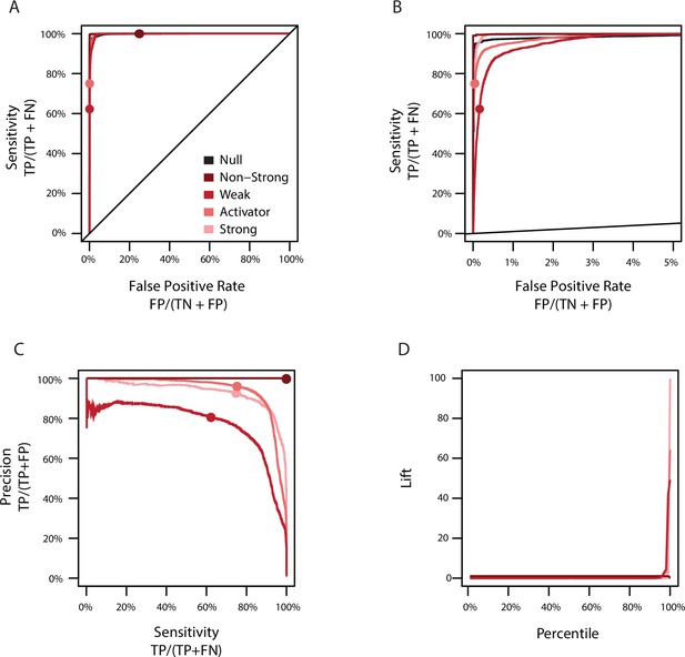
Model error rates and misclassification.
(A) Sensitivity versus the false positive rate of the full model for each classification. The non-strong class (dark red) consists of genotypes labeled as either null (black) or weak (red); the activator class (light red) consists of genotypes labeled as weak or strong (pink). Sensitivity is the percent of genotypes correctly estimated to be in a class (TP) among the set of all genotypes originally assigned to that class (TP + FN). The false positive rate is the percent of genotypes incorrectly estimated to be in a class (FP) among the set of all genotypes not originally assigned to that class (TN+FP). Circles show the sensitivity and false positive rate in the full model. (B) Same as A, showing a reduced portion of the x-axis. (C) Precision versus sensitivity of the full model for each classification. Colors are the same as C. Precision is the percent of genotypes correctly estimated to be in a class (TP) among the set of all genotypes estimated to be in that class (TP + FP). (F) Lift of each percentile for each classification. Genotypes were ordered by genetic score and lift calculated as the frequency of each class in a percentile relative to the average frequency of each class in the entire data set.
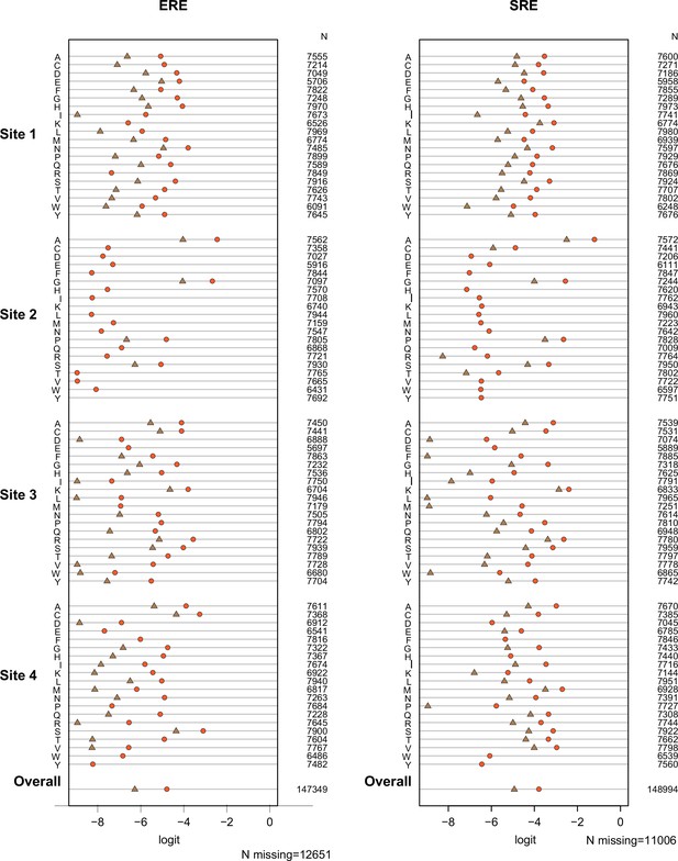
Test of proportional odds assumption.
Each panel shows estimated main-effect coefficients for each amino acid at the variable sites using simple logistic regression, when the activation class of variants was coded in two different ways: null vs.weak+strong (brown), or null+weak vs. strong (orange). Under the proportional odds assumption, the difference between the two estimates should be the same across coefficients. Coefficients for the effect on ERE and SRE were estimated separately, and no epistasis was included in this preliminary model. Missing symbols indicate amino acid states never observed among strong activators (no brown) or only observed in null activators (no orange or brown). N gives the number of genotypes containing the specified state for which mean fluorescence values. The weighted average of all estimated coefficients is shown at the bottom.
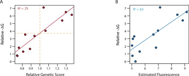
Model fit and ΔG of binding.
(A) ΔG relative to the weakest binder as estimated from fluorescence polarization versus the estimated genetic score. Genetic scores are scaled relative to the threshold to be a strong binder (vertical orange dashed line), with zero being the average genetic score of all genotypes. Dashed horizontal line shows the ΔG values estimated to correspond to this threshold by fitting a linear model (solid red line). (B) ΔG from fluorescence polarization versus the observed mean fluorescence of each genotype prior to categorization. Linear regression between ΔG and mean fluorescence (solid blue line).
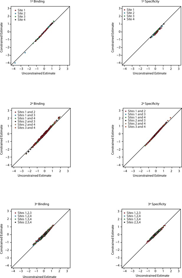
Model constrained estimates.
Unconstrained (x-axis) and constrained (y-axis) estimates for all coefficients in the third order model. Each panel is for a particular order of epistasis and either binding or specificity. Colors indicate the site, or combination of sites, for each set of coefficients.
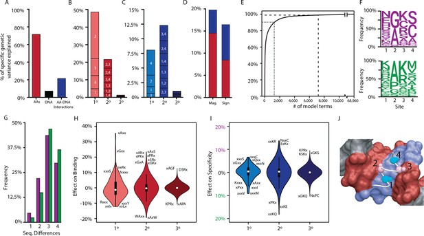
Genetic variance explained by components of the model.
(A) Fraction of genetic variance explained by all terms in the protein’s amino acid sequence (non-RE-specific binding, red), the RE’s DNA sequence (black), or the interaction between them (specificity, blue). (B) Fraction of genetic variance explained by terms in each model order for non-RE-specific binding. Indexes within each column show the variance explained by terms at each site or combination of sites. (C) Fraction of genetic variance explained by specificity terms at each order. (D) Fraction of genetic variance explained by pairwise epistatic effects that affect only the magnitude or affect the sign of interaction between two states; red and blue, effects on pairwise binding and specificity. (E) Cumulative fraction of genetic variance explained by model terms, ordered by the fraction of variance explained by each. Dashed lines indicate 90% and 99% of the total variance in genetic score explained by the complete model. (F) Frequency of amino acid states among sequences predicted to be strong activators on ERE (purple) and SRE (green). (G) Distribution of amino acid differences among predicted strong activator sequences on ERE (purple) and SRE (green). (H) Distributions of effect sizes on non-RE-specific binding. Largest-magnitude effects are labeled by amino acid state (x, any state). (I) Distribution of effect sizes on RE specificity. (J) Structural view of DBD recognition helix (white tube) and DNA response elements (surface). Blue, nucleotides that differ between ERE and SRE; red, nucleotides identical between ERE and SRE; gray, nucleotides outside of RE. Cα and Cβ atoms of variable residues in the recognition helix are shown as large and small spheres, respectively (cyan, largest effects on RE specificity; pink, largest effects on non-RE-specific binding). Coordinates are from the X-ray crystal structure of AncSR1-DBD, PDB 4OLN.
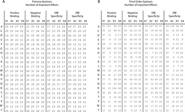
Number of important coefficients.
(A) Number of pairwise interaction terms involving each amino acid (rows) at each site (columns) that are needed to explain 99% of the full model specific genetic variance for positive binding, negative binding, ERE specificity, and SRE specificity. In each case, an amino acid can be involved in a maximum of 60 interactions (20 at each of the other three sites). (B) Same as left, but for third-order interactions. Each amino acid can be involved in a maximum of 1200 interactions (400 at each pair of the other three sites).
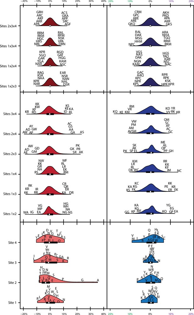
Variance explained of model coefficients for full model.
Distribution of effects for each site/site combination for the full model (1°+2°+3°). Effects are scaled to the value needed to be a strong binder. Binding effects (red) and specificity effects (blue) are separated. For main effects (light, bottom), all 20 amino acids are shown with single letter codes. For pairwise epistatic effects (medium, middle) and third-order effects (dark, top), only the most extreme five values for each site combination are shown.
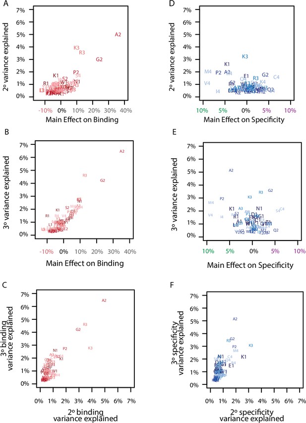
Correlation among model coefficients.
(A) Comparison of the main effect of each amino acid on binding with its epistatic effects on binding. Each point is a different amino acid (letter) at a different site (number). Each site is a different color from dark (site 1) to light (site 4). (B) Same as A, but for third-order interactions. (C) Same as A, but for the comparison of pairwise and third-order binding effects. (D) Comparison of the main effect of each amino acid on specificity with its epistatic effects on specificity. Each point is a different amino acid (letter) at a different site (number). Each site is a different color from dark (site 1) to light (site 4). (E) Same as D, but for third-order interactions. (F) Same as D, but for the comparison of pairwise and third-order specificity effects.
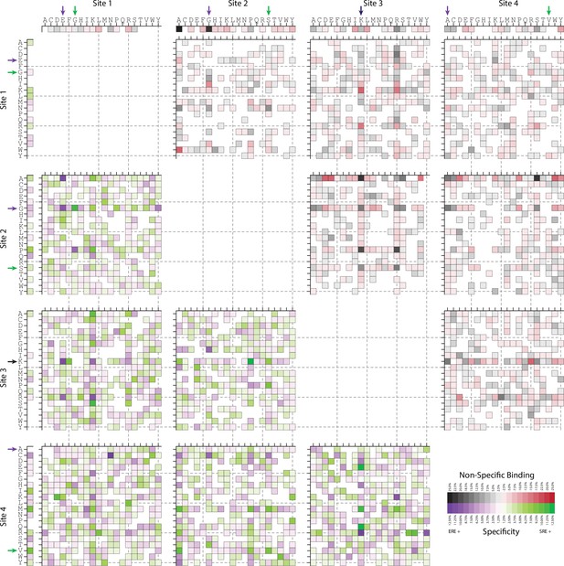
Model coefficients for first and second order.
First- and second-order effects on non-RE-specific binding (above the diagonal) and on specificity (below) for all amino acid sites and pairs. Effects are scaled relative to the value necessary to be classified as a strong binder. Arrows indicate the states found among extant steroid receptors (purple, estrogen receptors; green, ketosteroid receptors; black, both categories).
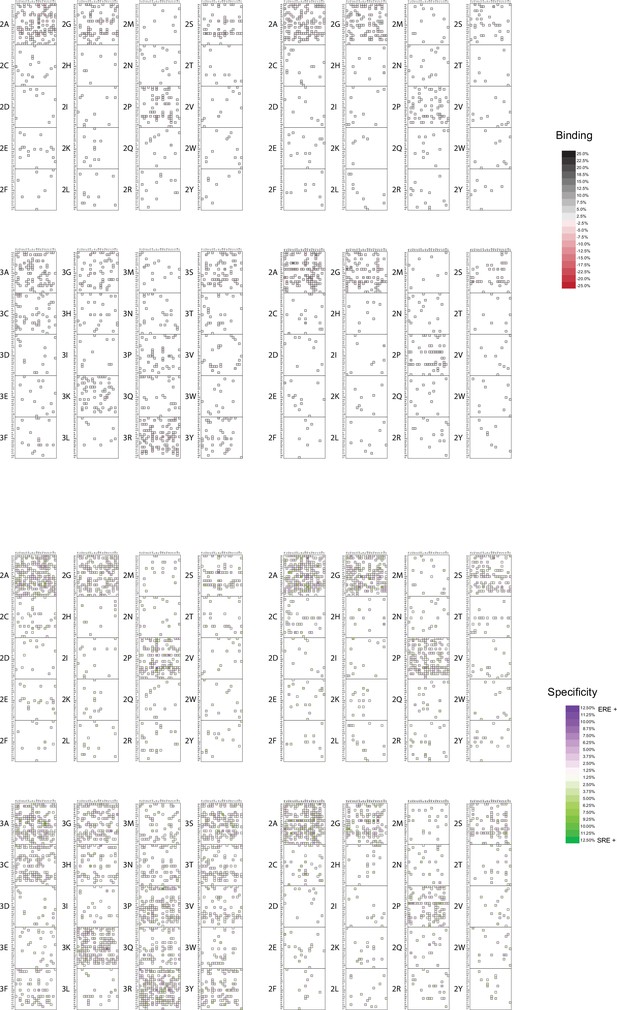
Model coefficients for third order.
Third-order epistatic effects for binding (top) and specificity (bottom). Effects that increase binding (black), decrease binding (red), prefer ERE (purple) and prefer SRE (green) are shown, with intensity corresponding to strength of effect. All effects are scaled relative to the value necessary to be classified as a strong binder. Scale is the same as Figure 2—figure supplement 4 for comparison. The majority of third-order terms are estimated as near zero and not shown.
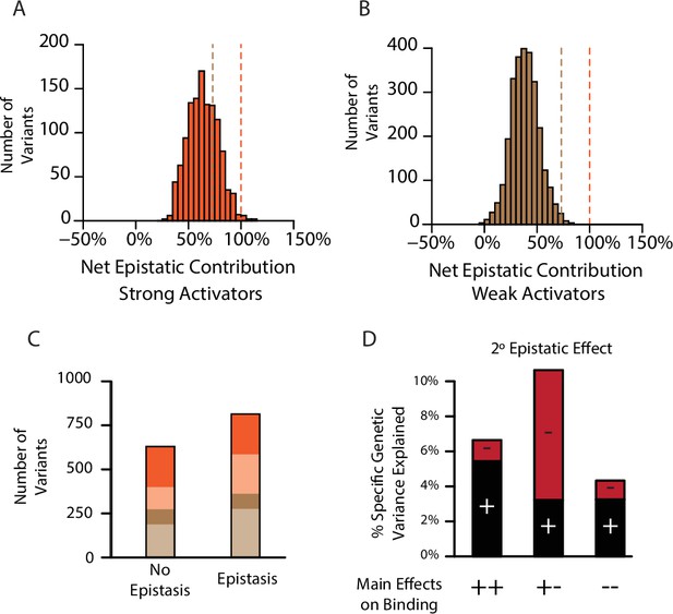
Pervasive pairwise epistasis.
(A) Net contribution of second- and third-order epistatic effects to the total genetic score of all variants predicted to be strong binders, scaled relative to the threshold for classification as a strong binder. Dashed lines, thresholds between activation classes. (B) Same as A, but for variants predicted as weak binders. (C) Number of variants classified as a weak (brown) or strong (orange) binder using terms from a model fit with no epistasis (1° effects only, left) or the full model with epistasis (1°+2°+3° effects, right). Dark colors represent the number of variants that retain the same class membership in both models; pale colors change class. (D) Percent of genetic variance explained by positive (black) and negative (red) pairwise binding interactions, classified by the sign of the main effects of the states.

Net contribution of third-order epistasis to binding.
(A) Net contribution of third-order epistatic effects to the total genetic score of all predicted strong binders. Dashed lines are the thresholds where net third-order epistatic effects are sufficient for a genotype to be classified as a weak (brown) or strong (orange) binder. (B) Same as A, but for predicted weak binders.

Genotype classifications across models.
Variants classified as a non (white), weak (brown), or strong (orange) binder in a model without epistasis (1°, left), the model with pairwise epistasis (1°+2°, middle), or the full model with epistasis (1°+2°+3° effects, right). Solid colors in skinny bars are genotypes that retain the same class membership as epistatic effects are added (to the right of a bar) or removed (to the left of a bar); pale colors indicate genotypes that change class membership and what class they are changed to.
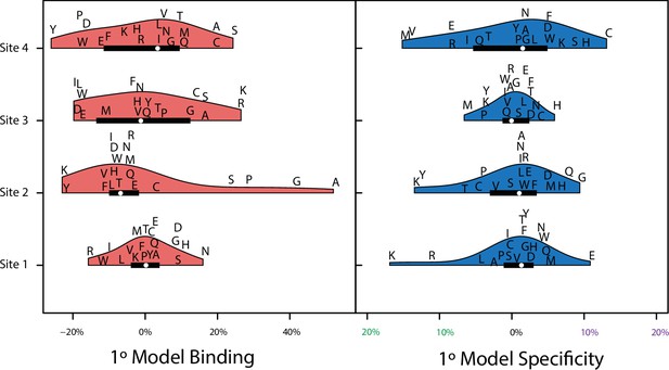
Variance explained of model coefficients for non-epistatic model.
Distribution of effects for each site for the main effect only model (1°). Effects are scaled to the value needed to be a strong binder. Binding effects (red) and specificity effects (blue) are separated.

Variance explained by non-specific third order epistasis.
Percent of specific genetic variance explained by positive (black) and negative (red) third-order binding interactions when main effects are positive (++), both are negative (--), or the main effects are of opposite signs (+-).
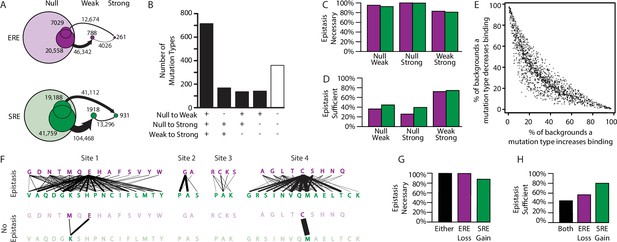
Effect of epistasis on the effects of mutations.
(A) Number of mutations that can promote protein variants from one activation class to another (circles). Each mutation is a single-amino-acid change from one unique sequence into another. (B) Effects on activation class of variants by unique mutation types (a change from one amino acid state to another at a particular site, irrespective of the background at other sites). Each column shows the number of mutation types that do (+) or do not (-) promote one or more variants from one class to another. (C, D) Of mutations that change a variant’s binding class, the fraction is shown for which the contribution of epistasis is necessary (C) and/or sufficient (D) to cross the threshold for reclassification. (E) Context-dependence of mutation effects. Fraction of genetic backgrounds in which a mutation type increases (x-axis) or decreases (y-axis) genetic score. Only mutations that change the genetic score by at least 5% of the threshold to be a strong activator are included. (F) Single-amino-acid mutations that change DNA specificity from ERE to SRE in the complete model (top) or the first-order-only model (bottom). Lines show mutations from the state in an ERE-specific variant (purple) to that in the SRE-specific variant (green); thickness is proportional to the number of backgrounds at other sites against which the mutation changes specificity. (G, H) Of mutations that change RE specificity, the fraction for which epistasis is necessary (G) and/or sufficient (H) to lose ERE binding (purple), gain SRE binding (green) or both (black).
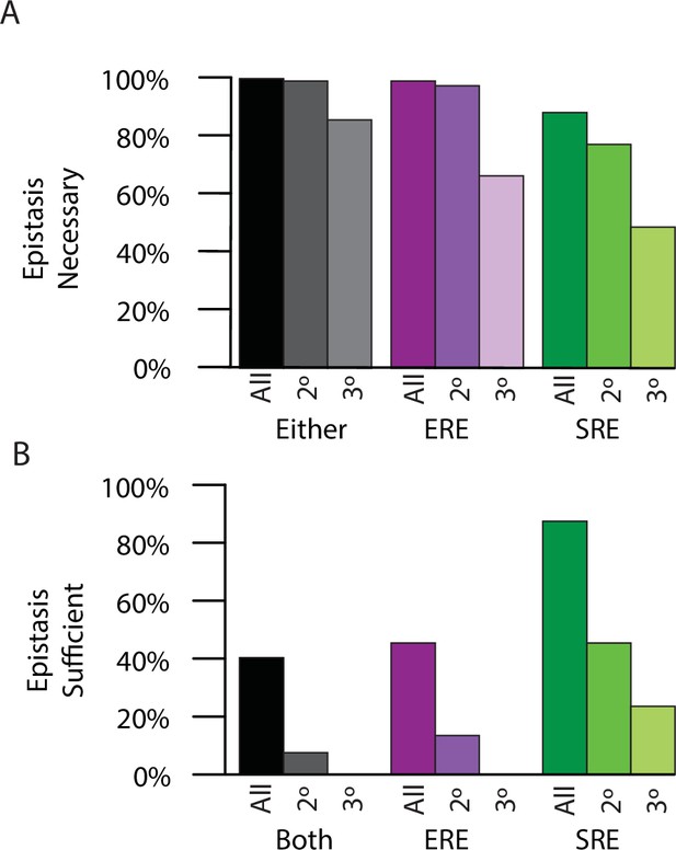
Necessity and sufficiency of epistasis.
(A) Percent of time epistasis is necessary for transition in specificity for the loss of ERE binding activity (purple), the gain of SRE binding activity (green), or either change for either all epistasis (dark), only pairwise epistasis (middle), or only third-order epistasis (light). (B) Percent of time epistasis is sufficient for the loss of ERE binding activity (purple) and the gain of SRE binding activity (green), or both (black) for either all epistasis (dark), only pairwise epistasis (medium), or only third-order epistasis (light).

Single step mutations in the pairwise epistasis model.
Single step mutations which change DNA specificity in the presence of pairwise epistasis. The ERE-specific amino acid state (purple) is on top, with the SRE-specific amino acid state (green) on the bottom. Line thickness is proportional to the frequency that a mutation causes the change in specificity.
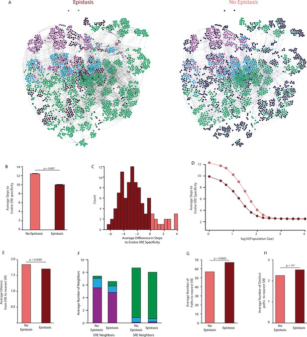
Effect of epistasis on the distribution of functions in sequence space.
(A) Force-directed graph of all variants that are predicted to be strong activators on one or both REs in the complete model (left) or the first-order-only model (right) after fitting to the DMS data. Lines connect variants that are separated by a single nucleotide change given the standard genetic code. Nodes are colored by their predicted functions given each model: strong activator on ERE (purple), SRE (green), or both (cyan); black nodes are null but predicted to be a strong activator under the other model. Nodes that are null in both models are excluded from the network. (B) Average number of steps in sequence space for each ERE-specific genotype to reach an SRE-specific genotype when evolution is simulated using a model with only purifying selection and drift. Error bars, 95% confidence interval based on 100 replicates per starting point. (C) Distribution of the average difference in steps needed to reach an SRE-specific variant from each ERE-specific variant when epistasis is included or excluded, using the same evolutionary process as in B. Light and dark bars show cases in which epistasis makes the path shorter or longer, respectively, from a given ERE-specific variant. (D) Average number of steps needed to reach an SRE-specific genotype from each ERE-specific genotype in the sequence space of the complete (dark line) and first-order model (light line), when evolution is simulated with positive selection for increased SRE specificity. The “population size” parameter controls the strength of positive selection relative to drift. (E) Average distance from each ERE-specific variant to the closest SRE-specific genotype in the sequence space of the first-order and complete models. (F) Average number of single-step neighbors in sequence space per node that is ERE-specific (left) or SRE-specific (right), in the presence or absence of epistasis. Each column shows the average number of neighbors adjacent to the designated node that are strong activators on ERE (purple), SRE (green), or both (cyan). (G) Average number of unique minimum length paths connecting ERE-specific variants to their nearest SRE-specific neighbor in the first-order and complete models. (H) Same as G for distinct minimum length paths. All p-values were calculated from a permutation test.
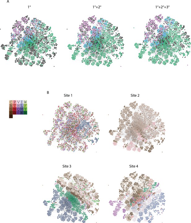
Distribution of genotypes and states in sequence space.
(A) Force directed graph of genotypes that are activators in either the absence of epistasis (left), the presence of pairwise epistasis, or both pairwise and third-order epistasis (right). In each case, each node is a genotype, colored by if it is ERE-specific (purple), SRE-specific (green), promiscuous (blue), or a non-binder in the network but an activator in one of the other networks (black). All activator nodes are connected in a given network based on single amino acid changes via the genetic code. (B) Amino acid state at each node in the force directed graph for each site. Amino acids are colored to reveal clustering in the force directed graph and are labeled by single letter codes. S and Z are used to represent the two non-connected regions of the genetic code containing serine codons.
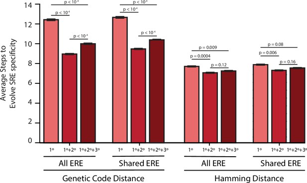
Evolutionary distances with purifying selection.
Average number of steps needed to reach an SRE-specific genotype from an ERE-specific genotype in the absence of epistasis (left, light), the presence of pairwise epistasis (middle), or both pairwise and third-order epistasis (right, dark) in a model with no positive selection for function. Error bars give a 95% confidence interval on the estimate based on 100 replicates from each ERE-specific genotype. Values are shown for either all ERE-specific starting genotypes or only ERE-specific genotypes found in all three networks when genotypes are connected via either the genetic code or by hamming distance. All p-values were calculated from a permutation test.
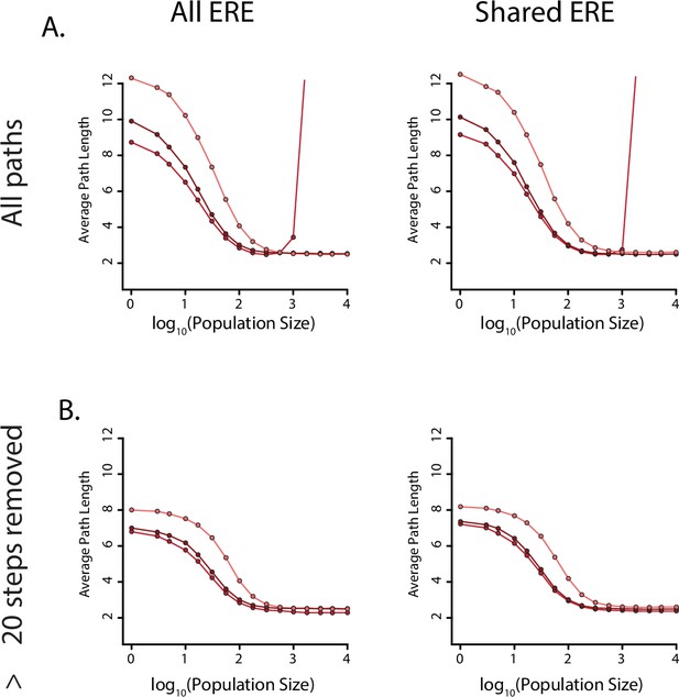
Evolutionary distances with positive selection for specificity.
(A) Average number of steps needed to reach an SRE-specific genotype from an ERE-specific genotype in the absence of epistasis (light), the presence of pairwise epistasis (middle), or both pairwise and third-order epistasis (dark) in a model with positive selection for increased SRE specificity for all ERE-specific starting genotypes (left) or shared ERE-specific genotypes found in all three networks (right). The population size was varied to control the relative strength of positive selection. (B) Same as A, but after removing paths that are greater than 20 steps long.
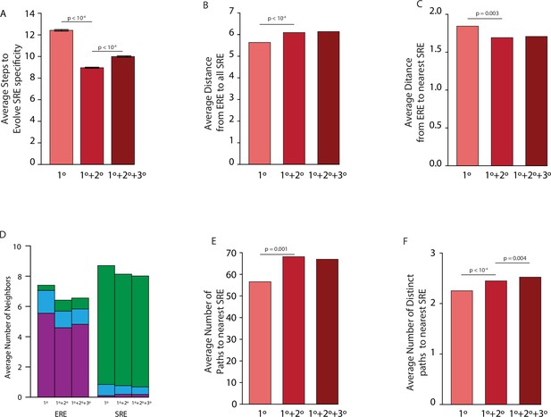
Effect of epistasis on distribution of functions in sequence space for all models.
(A) Average number of steps needed to reach an SRE-specific genotype from an ERE-specific genotype in the absence of epistasis (left, light), the presence of pairwise epistasis (middle), or both pairwise and third-order epistasis (right, dark) in a model with no positive selection for function. Error bars give a 95% confidence interval on the estimate based on 100 replicates from each ERE-specific genotype. (B) Average distance between all ERE-specific genotypes and all SRE-specific genotypes in the absence of epistasis (left, light), the presence of pairwise epistasis (middle), or both pairwise and third-order epistasis (right, dark). (C) Average distance between all ERE-specific genotypes and the closest SRE-specific genotype in the absence of epistasis (left, light), the presence of pairwise epistasis (middle), or both pairwise and third-order epistasis (right, dark). (D) Average number of single step neighbors for ERE-specific (left) and SRE-specific (right) genotypes in the absence of epistasis (left, light), the presence of pairwise epistasis (middle), or both pairwise and third-order epistasis (right, dark). In each case, the average number of neighbors that are ERE-specific (purple), promiscuous (blue), or SRE-specific (green) are shown. (E) Average number of shortest paths between all ERE-specific and nearest SRE-specific genotype in the absence of epistasis (left, left), the presence of pairwise epistasis (middle), or both pairwise and third-order epistasis (right, dark). (F) Average number of distinct shortest paths between all ERE-specific and nearest SRE-specific genotype in the absence of epistasis (left, light), the presence of pairwise epistasis (middle), or both pairwise and third-order epistasis (right, dark). All p-values were calculated from a permutation test.

Genetic architecture of the historical change in RE specificity.
(A) Each intermediate on the set of direct paths from the RH sequence of AncSR1 (egKa) to AncSR2 (GSKV) is shown at a vertex of the cube. At each vertex, the total genetic score for binding ERE (right) and SRE (left) are shown, scaled to 100 as the threshold for strong activation, and colored dark if the variant is a strong activator on ERE (purple) and/or SRE (green). Contribution of terms to non-specific binding (top) and specificity (bottom, colored by the RE they favor) are shown. Lines connect genotypes that differ by a single amino acid mutation; solid lines connect vertices that are strong activators on one or both REs; dotted lines connect to a vertex that activates on neither RE. (B) Contribution of historical changes in state to the change in RE specificity. Each genotype along the plausible path from AncSR1 to AncSR2 RH is shown at left. For egKa and GSKV, the contribution of effects at each order to the total genetic score for non-RE-specific binding (top) and RE-specificity (bottom) is shown, scaled as in A. Each cell is shaded by the magnitude of the effect at that site or combinations, and the sum of effects for the category is shown at right. The middle rows show the effect of each amino acid mutation along the path, defined as the effect of the derived state (or combination) minus that of the ancestral state or combination. Solid outline, mutation that caused the initial acquisition of SRE binding; dashed outlines, mutations that changed the determinants of SRE binding. The RE column shows the global specificity effect. This value is constant during evolution, but is needed to reconstruct the specificity values shown in A.


