Mechanical coupling coordinates microtubule growth
- Department of Physiology & Biophysics, University of Washington, United States
- Basic Sciences Division, Fred Hutchinson Cancer Research Center, United States
Figures
Figure 1
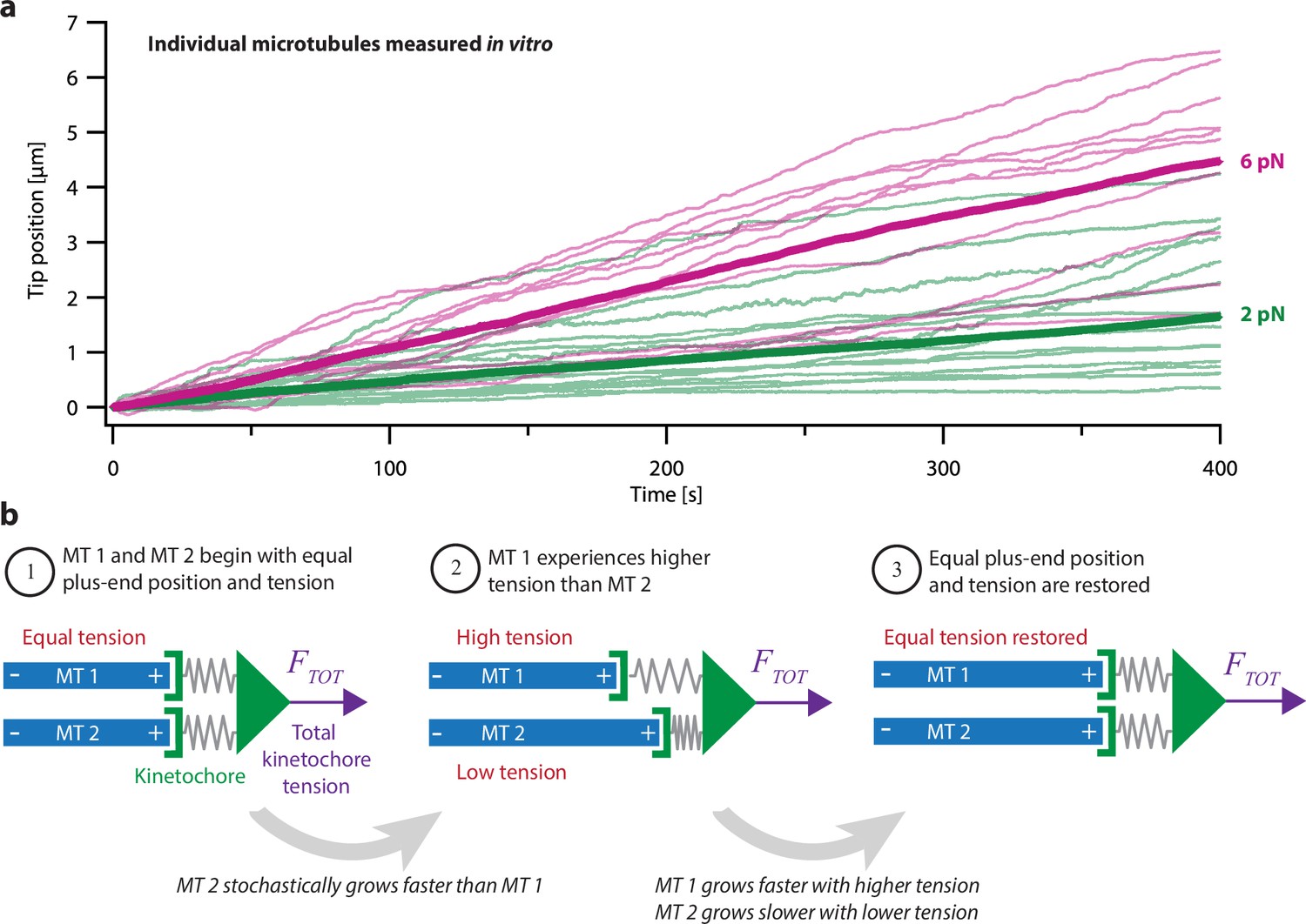
Intrinsic variability in microtubule growth could be coordinated by mechanical coupling.
(a) Microtubules (MTs) grow at intrinsically variable rates that increase with force, on average. Example recordings show plus-end position versus time for individual growing microtubules subject to a constant tensile force of either 2 or 6 pN (thin green or magenta traces, respectively). At each force, 10–14 example recordings are shown, together with the mean position versus time (thick traces, computed from N=25 or N=10 individual recordings at 2 or 6 pN, respectively). Individual traces are from Akiyoshi et al., 2010. (b) Mechanism by which mechanical coupling could coordinate growing microtubules. In this example, two microtubules share a total force, FTOT, through two spring-like connections to their plus-ends. If one microtubule stochastically lags behind, it will experience more tension than the leading microtubule due to differential stretching of their spring-connections. Because tension tends to accelerate plus-end growth (as illustrated in (a)), the higher tension will tend to accelerate the growth of the lagging microtubule, causing it to catch up.
Figure 2
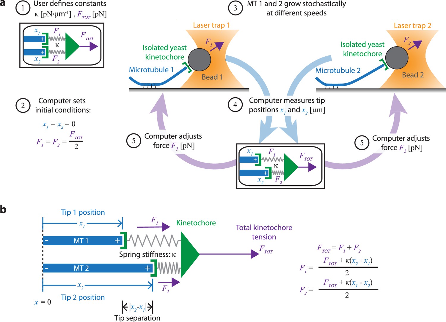
Dual-trap assay to measure the coordination of two real microtubules in vitro coupled together by simulated spring-like connections to a shared tensile load.
(a) Schematic of the dual-trap assay, which measures the effects of the spring-coupler model (detailed in (b)) on real microtubules (MTs) growing in vitro. Two dynamic microtubules are grown from seeds anchored to two separate coverslips on two separate stages, each with their own microscope and laser trap. Each laser trap applies tension to its respective microtubule plus-end via a bead decorated with isolated yeast kinetochores, and each tension is adjusted dynamically under feedback control by a shared computer. Initially (steps 1 and 2), microtubule plus-ends are considered to have the same position (x1=x2=0) so that each bears half of the total user-input tension (FTOT). Over time, as microtubules grow at different rates (step 3), the computer dynamically adjusts the tension on each microtubule according to the spring-coupler model (steps 4 and 5), so that the higher the tip separation (|x1 - x2|) and stiffness (ĸ), the larger the difference in tension between the two microtubules. (b) Spring-coupler model used to represent the physical connection between two microtubule plus-ends via a kinetochore. Both springs have identical stiffnesses (ĸ). The kinetochore is assumed to be in force equilibrium such that the sum of the spring forces is equal to the total external force, FTOT, which is kept constant in the current study.
Figure 3 with 1 supplement
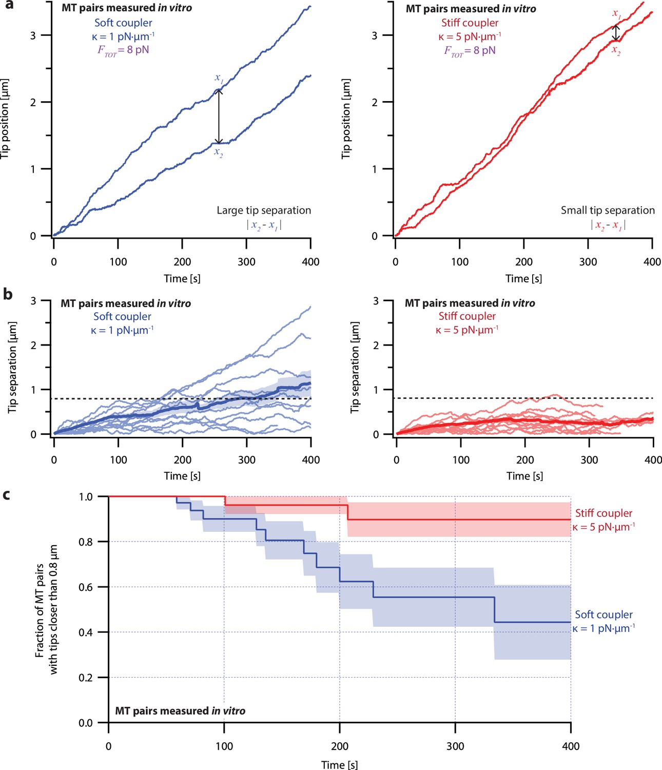
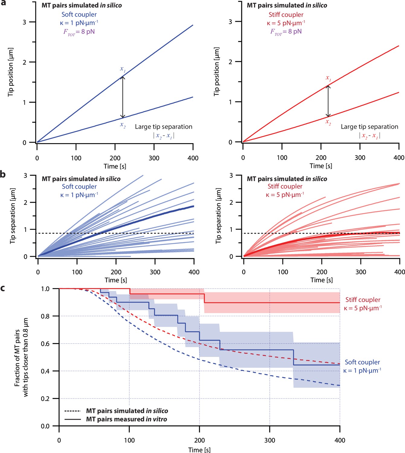
Microtubule pairs growing in vitro are coordinated by mechanical coupling.
(a) Example dual-trap assay recordings showing real microtubule (MT) plus-end positions over time for representative microtubule pairs coupled via soft (1 pN·µm–1, left) or stiff (5 pN·µm–1, right) simulated spring-couplers. All dual-trap data was recorded with FTOT = 8 pN. (b) Tip separation (|x1 - x2|) between microtubule plus-end pairs that were coupled with either soft (left) or stiff (right) simulated spring-couplers over 400 s of growth. Light colors show tip separations for 10 individual microtubule pairs with each coupler stiffness, while dark colors show mean tip separation for all recorded pairs (N=50 and N=43 recordings with soft and stiff couplers, respectively). (c) Fraction of microtubule pairs whose plus-ends remained within 0.8 µm of each other over time. (In other words, the fraction of pairs at any given time whose tip separation had not exceeded the dashed line in (b).) Shaded regions in (b) and (c) show SEMs from N=50 and N=43 recordings with soft and stiff couplers, respectively.
Figure 3—figure supplement 1
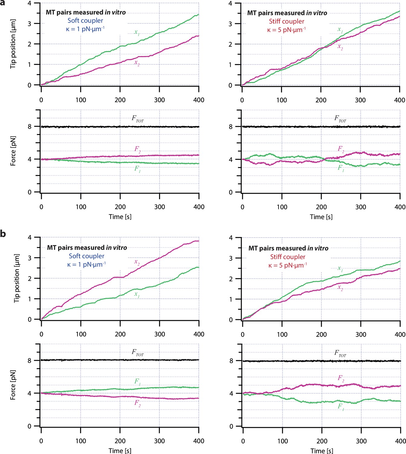
Additional dual-trap assay recordings showing tip positions and forces on pairs of growing microtubules.
(a) Example dual-trap assay recordings showing real microtubule (MT) plus-end positions (top) and forces (bottom) plotted against time for representative microtubule pairs coupled via soft or stiff simulated spring-couplers. Plus-end position data in the top graphs is recopied from Figure 3a. Black traces in the bottom graphs show total force on the two microtubules (FTOT) and demonstrate that a constant total force of FTOT = 8 pN was maintained by the feedback-control. (b) Two additional examples of dual-trap assay recordings, formatted as in (a).
Figure 4
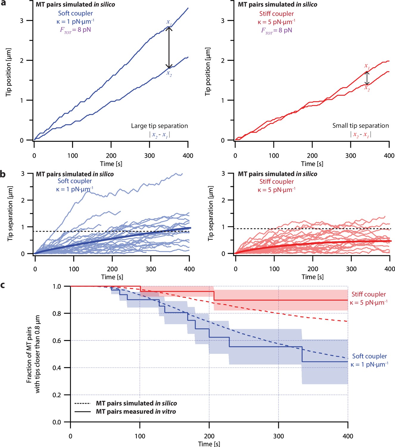
Simple non-pausing simulations fail to recapitulate the coordinated growth of mechanically coupled microtubule pairs.
(a) Example simulations of microtubule (MT) plus-end positions over time using the non-pausing model. Simulated microtubule pairs were coupled via soft or stiff spring-couplers and shared a total load FTOT = 8 pN to match dual-trap assay conditions. (b) Tip separations between microtubule plus-end pairs that were simulated using the non-pausing model and coupled with either soft (left) or stiff (right) spring-couplers. Light colors show tip separations for N=40 individual simulated microtubule pairs, while dark colors show mean tip separation for N=10,000 simulated pairs. (c) Comparison between the fraction of in silico (simulated, dashed curves) and in vitro (real, solid curves) microtubule pairs whose plus-ends remained within 0.8 μm of each other over time. Shaded regions show SEMs from N=50 and N=43 in vitro recordings with soft and stiff couplers, respectively. Soft- and stiff-coupled microtubule pairs were each simulated N=10,000 times over 400 s of growth in both (b) and (c). Simulation parameters for (a), (b), and (c) can be found in Table 1.
Figure 5 with 2 supplements
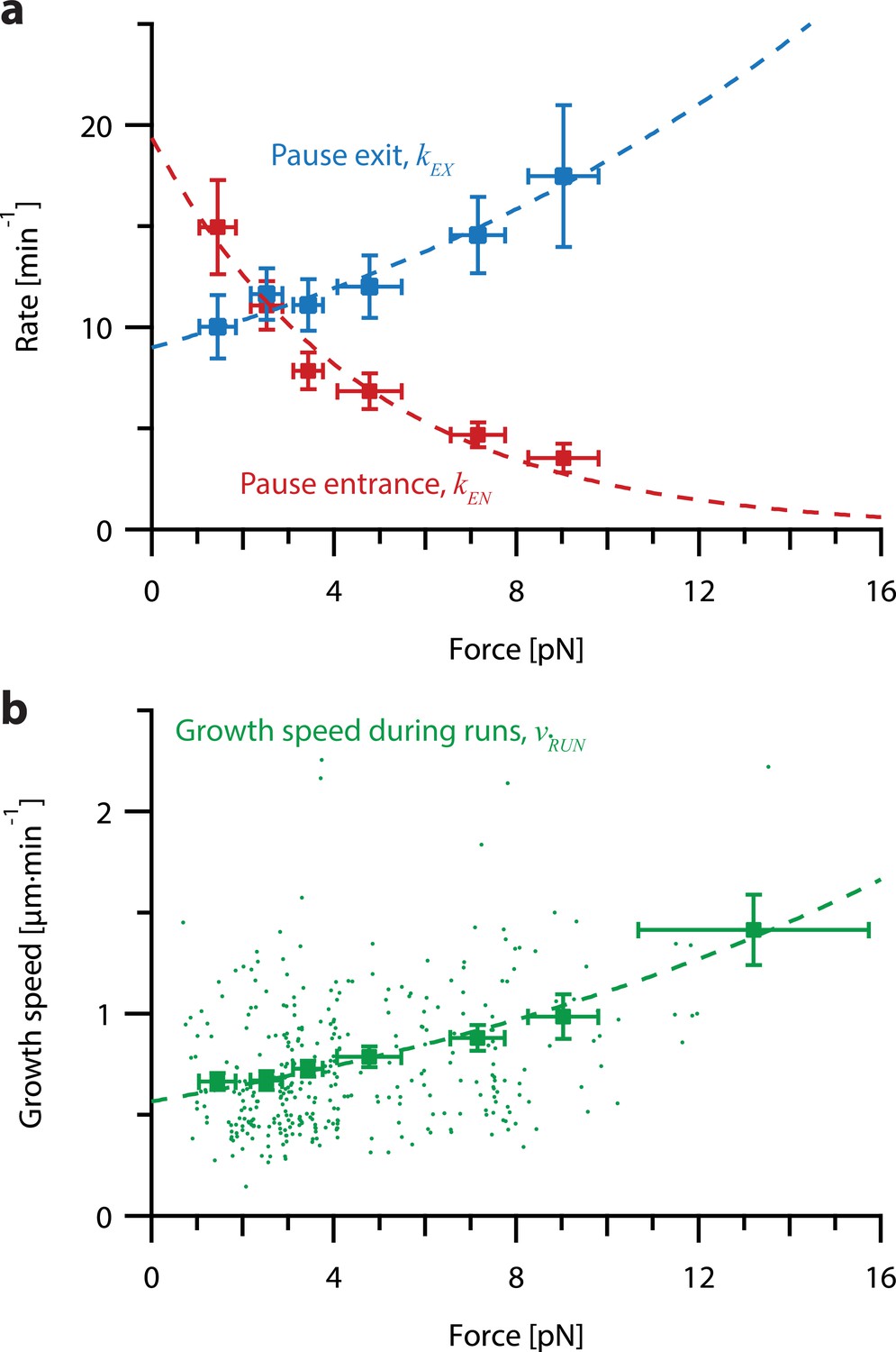
Increasing tension on individual growing microtubules suppresses pausing and accelerates growth during runs.
(a) As tension increases on a growing microtubule tip, the rate of pause entrance decreases, while the rate of pause exit increases. Mean pause entrance and exit rates (kEN and kEX) were estimated as described in Figure 5—figure supplement 1 and are plotted as functions of force. Error bars show counting uncertainties from N=25–85 individual microtubule recordings and dashed curves show least squares exponential fits. (b) As tension on a microtubule tip increases, the growth during runs (i.e. in-between pauses) is accelerated. Points show run speeds measured from recordings of individual microtubules subject to constant tensile forces (from Akiyoshi et al., 2010). Symbols represent mean run speeds (vRUN) grouped according to the applied tensile force. Error bars show SEMs from N=9–85 individual microtubule recordings and dashed curve shows the least squares exponential fit. See Figure 5—figure supplement 1 and Methods for details and Table 1 for fit parameters.
Figure 5—figure supplement 1
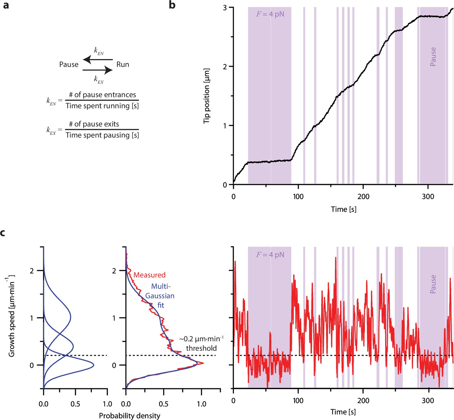
Individual microtubules frequently pause during periods of overall growth.
(a) Growing microtubules switch between states of ‘pause,’ when plus-end growth speed is nearly zero, and ‘run,’ when the plus-end is clearly growing. Pause entrance and exit rates, kEN and kEX, were quantified by counting the numbers of entrances or exits and dividing by the total amount of time spent in the run or pause states, respectively. (b) Example recording showing plus-end position versus time for an individual microtubule subject to a constant tensile force of 4 pN and exhibiting frequent pauses (denoted by purple shaded regions). This example recording is one of N=356 force-clamp traces (from Akiyoshi et al., 2010) used to estimate the pause entrance and exit rates and growth speeds during runs as functions of force (as shown in Figure 5). (c) Classification of runs and pauses. Instantaneous growth speed was computed as a function of time (and plotted at right) from the recording shown in (b), using a 2 s sliding window, and then assembled into a histogram (middle plot, red) and fit with a sum of multiple Gaussian curves (middle and left plots, blue). One Gaussian was always centered at 0 µm·min–1 and defined as the ‘pause’ peak. The intersection of the pause peak and the Gaussian having the next highest mean growth speed was identified for each individual recording and used as a threshold (dashed horizontal line) to distinguish pauses and runs for that recording. Pauses were defined as periods longer than 1 s when the instantaneous growth speed fell below the threshold, while runs were defined as periods longer than 1 s when growth speed was above the threshold (see Methods for details).
Figure 5—figure supplement 2
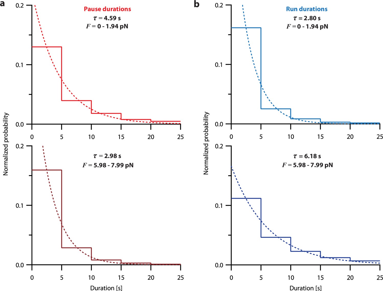
Pause and run durations are exponentially distributed.
(a) Normalized histograms showing pause durations measured from recordings of individual microtubules growing under constant levels of tension (force-clamp data from Akiyoshi et al., 2010), either between 0 and 2 pN (top), or between 6 and 8 pN (bottom), corresponding to the lowest and third-highest force bins in Table 2, respectively. (b) Normalized histograms showing run durations measured from recordings of individual microtubules growing under constant levels of tension (force-clamp data from Akiyoshi et al., 2010), as in (a). For both (a) and (b), least-squares regressions are shown as dashed curves. The indicated time constants (τ) were derived from these fits.
Figure 6 with 4 supplements
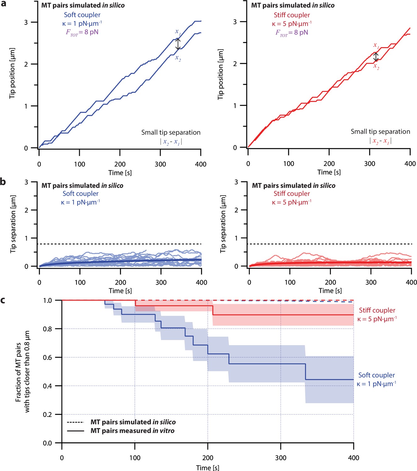
Simulations recapitulate the coordinated growth of mechanically coupled microtubule pairs.
(a) Example simulations of microtubule (MT) plus-end positions over time using the pausing model. Simulated microtubule pairs were coupled via soft or stiff spring-couplers and shared a total load FTOT = 8 pN to match dual-trap assay conditions. (b) Tip separations between microtubule plus-end pairs that were simulated using the pausing model and coupled with either soft (left) or stiff (right) spring-couplers. Light colors show tip separations for N=40 individual simulated microtubule pairs, while dark curves show mean tip separation for N=10,000 simulated pairs. (c) Comparison between the fraction of in silico (simulated, dashed curves) and in vitro (real, solid curves) microtubule pairs whose plus-ends remained within 0.8 μm of each other over time. Shaded regions show SEMs from N=50 and N=43 in vitro recordings with soft and stiff couplers, respectively. Soft- and stiff-coupled microtubule pairs were each simulated N=10,000 times over 400 s of growth in both (b) and (c). Simulation parameters for (a), (b), and (c) are listed in Table 1.
Figure 6—figure supplement 1
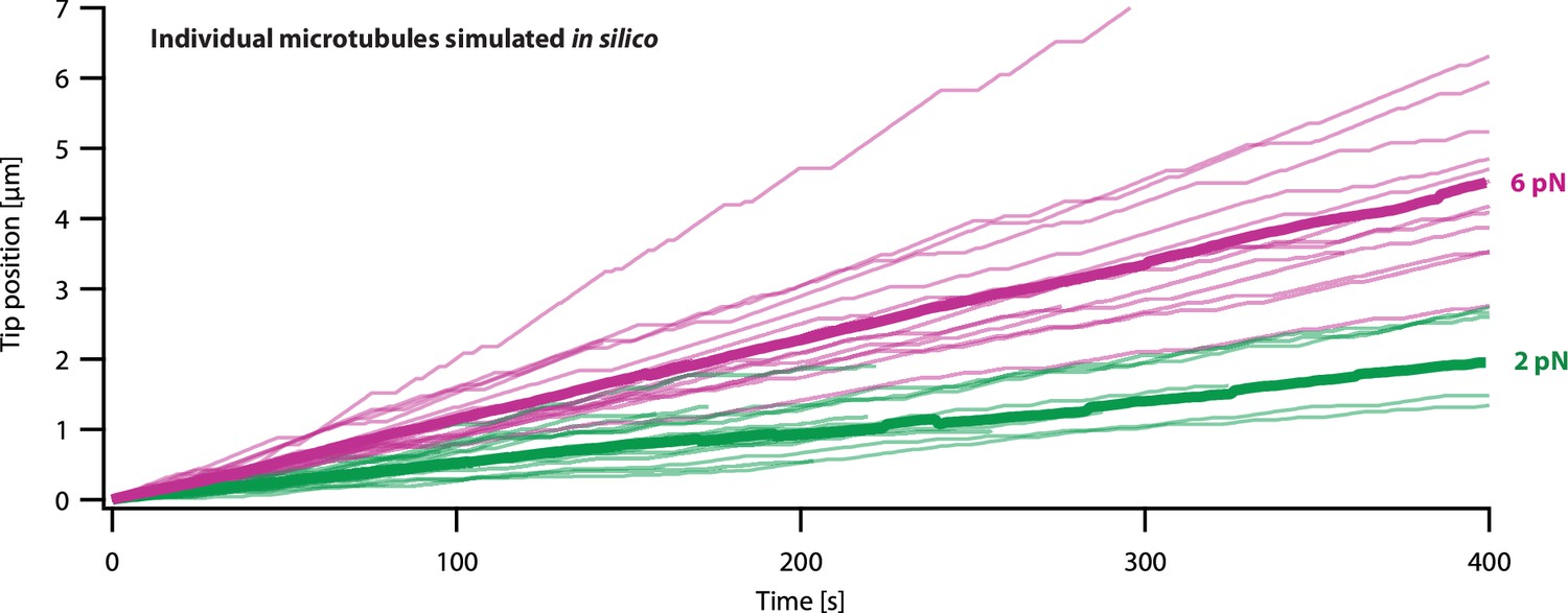
Simulations of microtubule growth under constant force using the pausing model resemble real microtubule recordings.
Examples using the pausing model to simulate plus-end position versus time for individual growing microtubules subject to a constant tensile force of either 2 or 6 pN (light green or magenta traces, respectively). At each force, N=16 example simulations are shown, together with the corresponding mean positions versus time (thick traces, computed from the N=16 individual simulations).
Figure 6—figure supplement 2
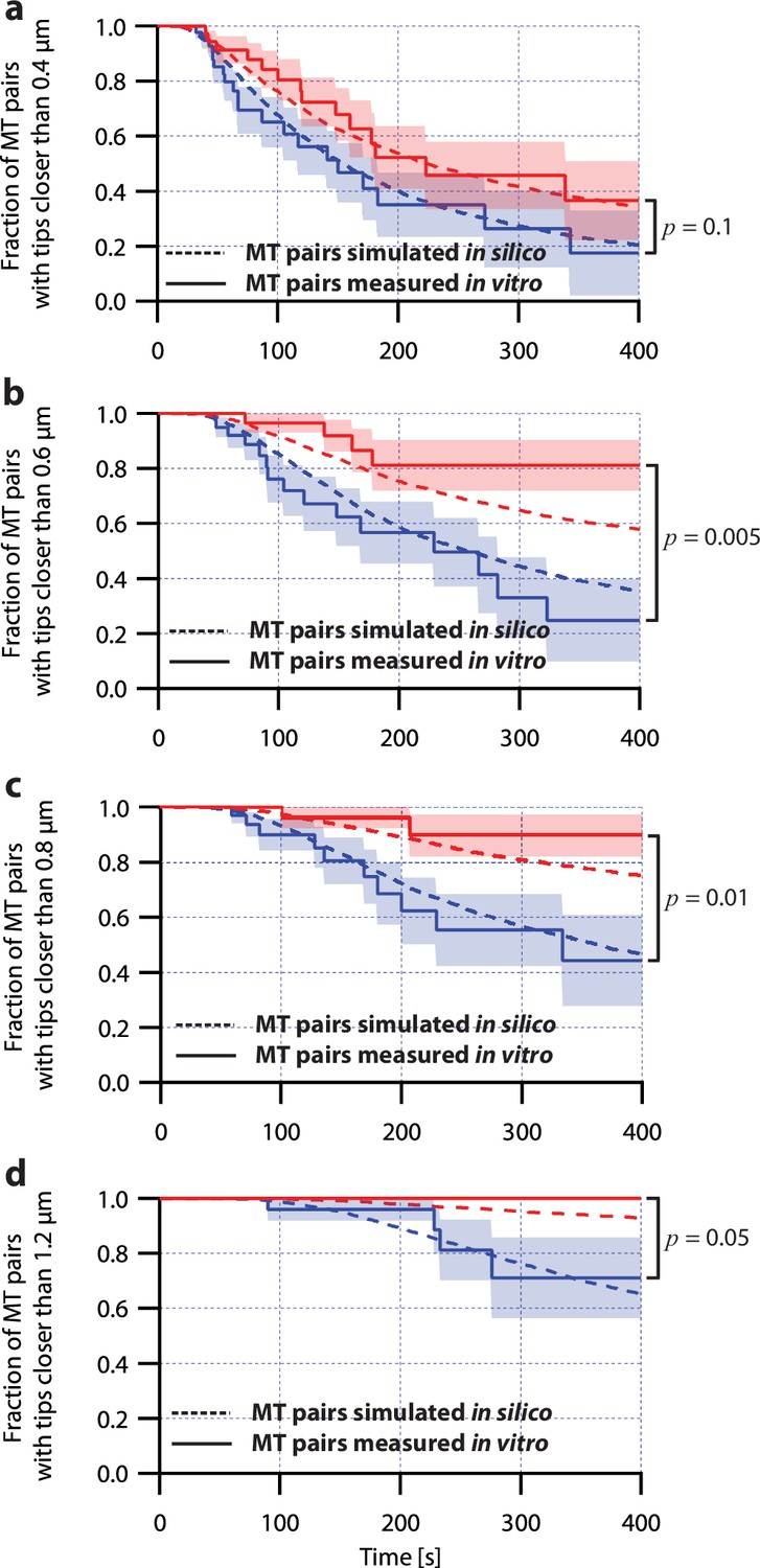
Simulations of microtubule pairs using the pausing model maintain tip separations similar to real microtubule pairs.
Comparison between the fraction of in silico (simulated, dashed curves) and in vitro (real, solid curves) microtubule (MT) pairs whose plus-ends remained within (a) 0.4 μm, (b) 0.6 μm, (c) 0.8 μm, and (d) 1.2 μm of each other over time. Microtubule pairs in silico and in vitro shared a total load of FTOT = 8 pN and were coupled via soft or stiff spring couplers. Shaded regions show SEM from N=50 and N=43 in vitro recordings with soft and stiff couplers, respectively. Soft- and stiff-coupled microtubule pairs were each simulated N=10,000 times over 400 s of growth. Simulation parameters can be found in Table 1. P-values indicate comparisons between soft- and stiff-coupled microtubule pairs in vitro using a log-rank test.
Figure 6—figure supplement 3
Simulations using an ergodic version of the pausing model, without intrinsic heterogeneity, fail to recapitulate the coordinated growth of mechanically coupled microtubules pairs.
(a) Example simulations of microtubule (MT) plus-end positions over time using the ergodic pausing model. Simulated microtubule pairs were coupled via soft or stiff spring-couplers and shared a total load FTOT = 8 pN to match dual-trap assay conditions. (b) Tip separations between microtubule plus-end pairs that were simulated using the ergodic pausing model and coupled with either soft (left) or stiff (right) spring-couplers. Light colors show tip separations for N=40 individual simulated microtubule pairs while dark colors show mean tip separation for N=10,000 simulated pairs. (c) Comparison between the fraction of in silico (simulated, dashed curves) and in vitro (real, solid curves) microtubule pairs whose plus-ends remained within 0.8 μm of each other over time. Shaded regions show SEMs from N=50 and N=43 in vitro recordings with soft and stiff couplers, respectively. Soft- and stiff-coupled microtubule pairs were each simulated N=10,000 times over 400 s of growth in both (b) and (c). Simulation parameters for (a), (b), and (c) can be found in Table 1. As expected, microtubule pairs simulated using this ergodic model remained much closer together than real microtubule pairs, rarely separating by more than 0.5 µm irrespective of coupler stiffness. After 300 s, the average tip separation for soft-coupled pairs was only 0.202±0.002 µm (mean ± SEM from N=10,000 simulations), barely different from the average tip separation for stiff-coupled pairs of 0.134±0.002 µm (mean ± SEM from N=10,000 simulations). Combined with the success of the non-ergodic pausing model in fitting our dual-trap data, this supports the idea that microtubule growth can be considered non-ergodic during our 400 s experiments.
Figure 6—figure supplement 4
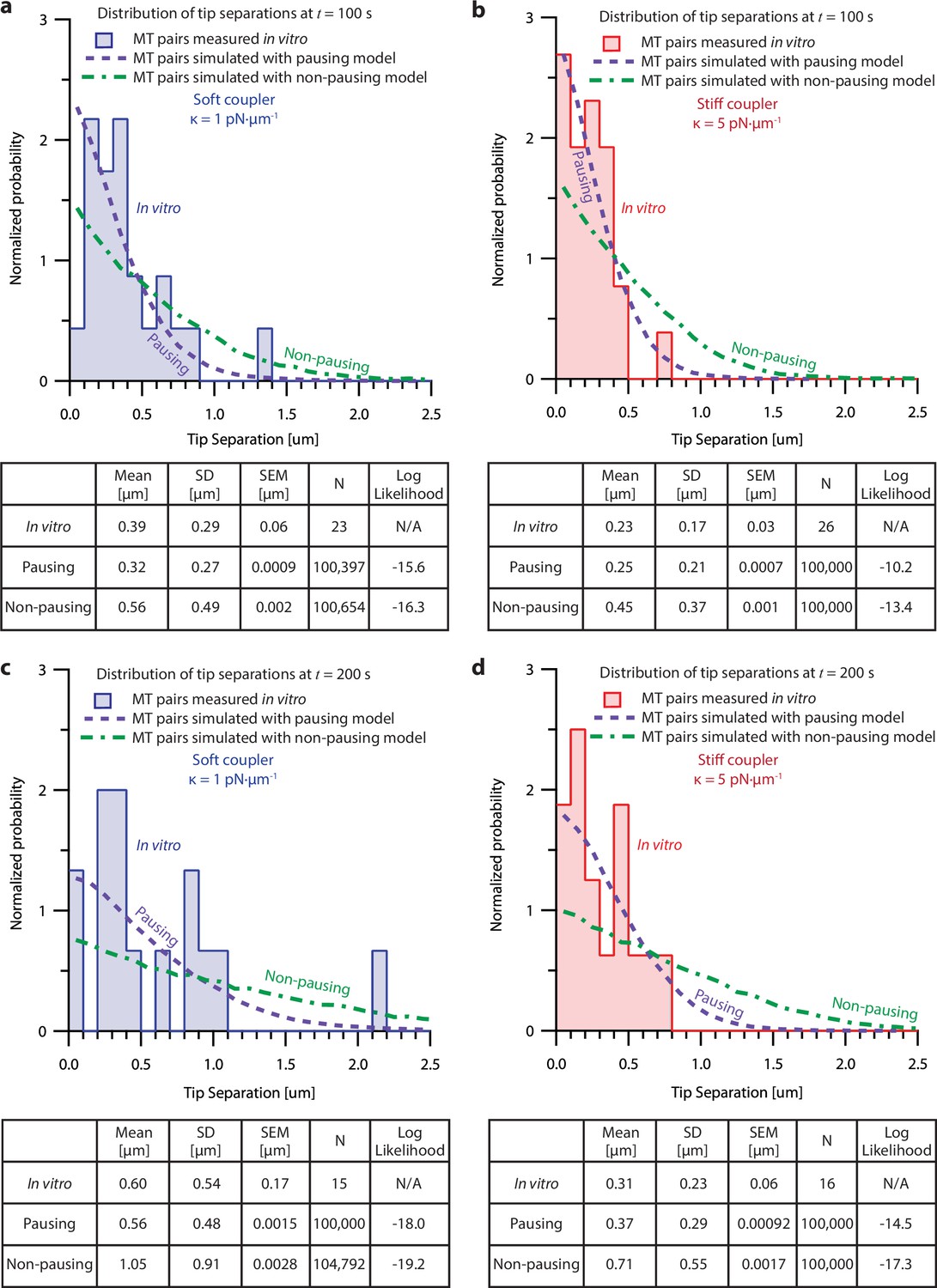
Probability analysis shows pausing model fits dual-trap recordings better than the non-pausing model.
(Top of each panel) Histograms of tip separation between microtubule pairs measured in the dual-trap assay and simulated using the pausing and non-pausing model. Soft-coupled pairs are shown on the left ((a) and (c)), while stiff-coupled pairs are shown on the right ((b) and (d)). Histograms of tip separations measured 100 s after the start of the recording or simulation are shown on the top ((a) and (b)), while tip separations measured 200 s after the start of the recording or simulation are shown on the bottom ((c) and (d)). Tip separation histograms produced by the pausing (purple) and non-pausing model (green) are represented with dashed lines, while dual-trap data is represented by bars. (Bottom of each panel) Tables comparing the means, standard deviations (SD), standard errors of the mean (SEM) and numbers of recordings (N) for in vitro microtubule pairs and microtubule pairs simulated using the pausing and non-pausing models. The log likelihood probability for each model given the in vitro data is shown in the righthand column. The greater the log likelihood, the greater the probability that the given model could reproduce the measured in vitro data. At both 100 s and 200 s, for soft and stiff couplers, the pausing model scores higher than the non-pausing model, indicating that the pausing model is a better fit to our in vitro data.
Tables
Table 1
Parameter table for coupled microtubule pairs simulated for non-pausing and pausing models.
Relevant parameters measured from constant force recordings from Akiyoshi et al., 2010. These parameters were used to simulate coupled microtubule pairs using each of the models described in the main text. The equation in which each parameter is used, as well as which models of microtubule growth use that parameter, are indicated.
| Parameter name | Parameter symbol | Relevant equation | Parameter estimate | Applicable models | Reference |
|---|---|---|---|---|---|
| Growth speed force sensitivity | 8.4 pN | non-pausing | Akiyoshi et al., 2010, Figure 4e | ||
| Unloaded pause entrance rate | 19.4 min–1 | pausing | Figure 5a, red | ||
| Pause entrance rate force sensitivity | –4.6 pN | pausing | Figure 5a, red | ||
| Unloaded pause exit rate | 9.0 min–1 | pausing | Figure 5a, blue | ||
| Pause exit rate force sensitivity | 14.1 pN | pausing | Figure 5a, blue | ||
| Unloaded run speed | 0.52 µm·min–1 | neither | Figure 5b | ||
| Run speed force sensitivity | 14.8 pN | pausing | Figure 5b |
Table 2
Number of recordings, bounds, and pause quantification from force-clamp dataset, binned by force.
Table describing constant force recordings in Akiyoshi et al., 2010 and the pause quantification performed in the current work. N indicates the number of recordings in a particular bin. For consistency, these force bins are identical to those used in Akiyoshi et al., 2010.
| Bin number | N | Lower bound [pN] | Upper bound [pN] | Pause entrances | Time in pause [s] | Pause exits | Time in run[s] |
|---|---|---|---|---|---|---|---|
| 1 | 41 | 0.69 | 1.94 | 1,834 | 10,957 | 1,830 | 7,364 |
| 2 | 85 | 1.94 | 2.97 | 3,502 | 18,047 | 3,501 | 18,952 |
| 3 | 77 | 2.97 | 3.999 | 2,376 | 12,842 | 2,374 | 18,159 |
| 4 | 60 | 3.999 | 5.98 | 1,937 | 9,661 | 1,932 | 16,993 |
| 5 | 60 | 5.98 | 7.99 | 1,439 | 5,930 | 1,438 | 18,465 |
| 6 | 25 | 7.99 | 10.3 | 387 | 1,298 | 378 | 6,559 |
| 7 | 9 | 10.3 | 18 | 23 | 93 | 23 | 712 |
Additional files
Download links
A two-part list of links to download the article, or parts of the article, in various formats.
Downloads (link to download the article as PDF)
Open citations (links to open the citations from this article in various online reference manager services)
Cite this article (links to download the citations from this article in formats compatible with various reference manager tools)
Mechanical coupling coordinates microtubule growth
eLife 12:RP89467.
https://doi.org/10.7554/eLife.89467.3


