A neuronal least-action principle for real-time learning in cortical circuits
- Department of Physiology, University of Bern, Switzerland
- Kirchhoff-Institute for Physics, Heidelberg University, Germany
- European Space Research and Technology Centre, European Space Agency, Netherlands
- Insel Data Science Center, University Hospital Bern, Switzerland
- Electrical Engineering, Yale University, United States
- MILA, University of Montreal, Canada
- Department of Computer Science, ETH Zurich, Switzerland
Figures
Figure 1
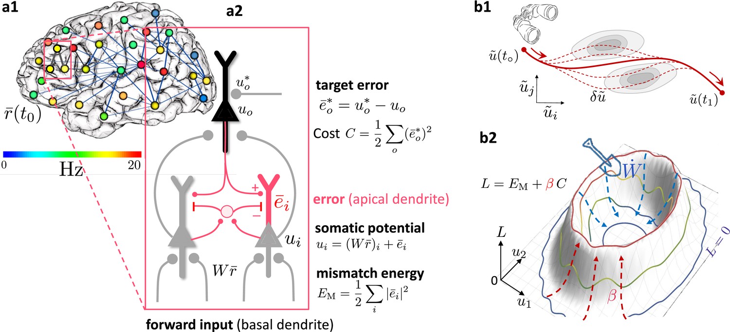
Somato-dendritic mismatch energies and the neuronal least-action (NLA) principle.
(a1) Sketch of a cross-cortical network of pyramidal neurons described by NLA. (a2) Correspondence between elements of NLA and biological observables such as membrane voltages and synaptic weights. (b1) The NLA principle postulates that small variations (dashed) of the trajectories (solid) leave the action invariant, . It is formulated in the look-ahead coordinates (symbolized by the spyglass) in which `hills' of the Lagrangian (shaded gray zones) are foreseen by the prospective voltage so that the trajectory can turn by early enough to surround them. (b2) In the absence of output nudging (), the trajectory is solely driven by the sensory input, and prediction errors and energies vanish (, outer blue trajectory at bottom). When nudging the output neurons towards a target voltage (), somatodendritic prediction errors appear, the energy increases (red dashed arrows symbolising the growing ‘volcano’) and the trajectory moves out of the hyperplanes, riding on top of the `volcano' (red trajectory). Synaptic plasticity reduces the somatodendritic mismatch along the trajectory by optimally ‘shoveling down the volcano’ (blue dashed arrows) while the trajectory settles in a new place on the hyperplane (inner blue trajectory at bottom).
Figure 2
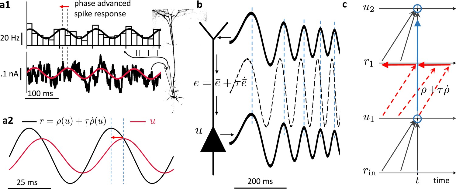
Prospective coding in cortical pyramidal neurons enables instantaneous voltage-to-voltage transfer.
(a1) The instantaneous spike rate of cortical pyramidal neurons (top) in response to sinusoidally modulated noisy input current (bottom) is phase-advanced with respect to the input adapted from Köndgen et al., 2008. (a2) Similiarly, in neuronal least-action (NLA), the instantaneous firing rate of a model neuron (, black) is phase-advanced with respect to the underlying voltage (, red, postulating that the low-pass filtered rate is a function of the voltage, ). (b) Dendritic input in the apical tree (here called ) is instantaneously causing a somatic voltage modulation (, modeling data from Ulrich, 2002). The low-pass filtering with along the dendritic shaft is compensated by a lookahead mechanism in the dendrite (). In (Ulrich, 2002) a phase advance is observed even with respect to the dendritic input current, not only the dendritic voltage, although only for slow modulations (as here). (c) While the voltage of the first neuron () integrates the input rates from the past (bottom black upward arrows), the output rate of that first neuron looks ahead in time, (red dashed arrows pointing into the future). The voltage of the second neuron () integrates the prospective rates (top black upwards arrows). By doing so, it inverts the lookahead operation, resulting in an instantaneous transfer from to (blue arrow and circles).
Figure 3
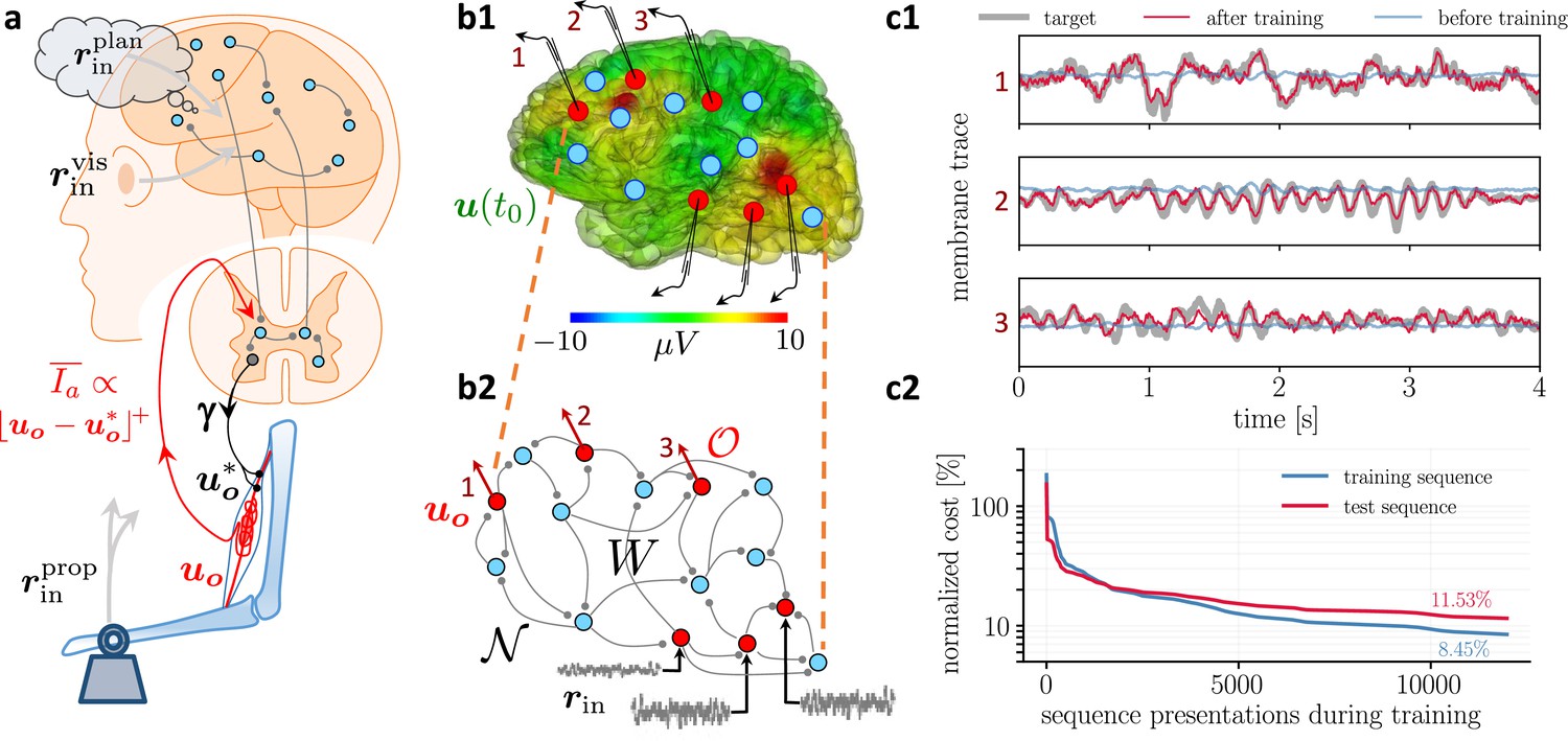
Moving equilibrium hypothesis for motor control and real-time learning of cortical activity.
(a) A voluntary movement trajectory can be specified by the target length of the muscles in time, , encoded through the -innervation of muscle spindles, and the deviation of the effective muscle lengths from the target, . The -afferents emerging from the spindles prospectively encode the error, so that their low-pass filtering is roughly proportional to the length deviation, truncated at zero (red). The moving equilibrium hypothesis states that the low-pass filtered input , composed of the movement plan and the sensory input (here encoding the state of the plant e.g., through visual and proprioceptive input, and ), together with the low-pass filtered error feedback from the spindles, , instantaneously generate the muscle lengths, , and are thus at any point in time in an instantaneous equilibrium (defined by Equation 7a, Equation 7b). (b1) Intracortical intracortical electroencephalogram (iEEG) activity recorded from 56 deep electrodes and projected to the brain surface. Red nodes symbolize the 56 iEEG recording sites modeled alternately as input or output neurons, and blue nodes symbolize the 40 ‘hidden’ neurons for which no data is available, but used to reproduce the iEEG activity. (b2) Corresponding NLA network. During training, the voltages of the output neurons were nudged by the iEEG targets (black input arrows, but for all red output neurons). During testing, nudging was removed for 14 out of these 56 neurons (here, represented by neurons 1, 2, 3). (c1) Voltage traces for the 3 example neurons in a2, before (blue) and after (red) training, overlaid with their iEEG target traces (gray). (c2) Total cost, integrated over a window of 8 s of the 56 output nodes during training with sequences of the same duration. The cost for the test sequences was evaluated on a 8 s window not used during training.
Figure 4
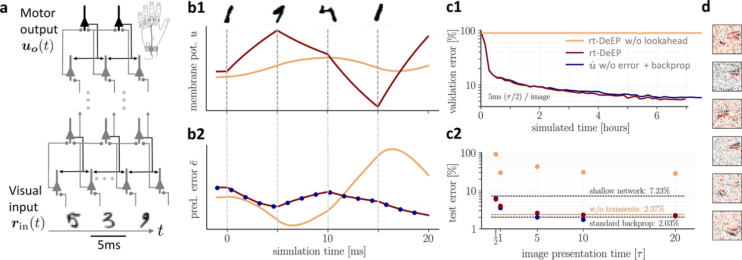
On-the-fly learning of finger responses to visual input with real-time dendritic error propagation (rt-DeEP).
(a) Functionally feedforward network with handwritten digits as visual input ( in Figure 3a, here from the MNIST data set, 5 ms presentation time per image), backprojections enabling credit assignment, and activity of the 10 output neurons interpreted as commands for the 10 fingers (forward architecture: 784×500×10 neurons). (b) Example voltage trace (b1) and local error (b2) of a hidden neuron in neuronal least-action (NLA) (red) compared to an equivalent network without lookahead rates (orange). Note that neither network achieves a steady state due to the extremely short input presentation times. Errors are calculated via exact backpropagation, i.e., by using the error backpropagation algorithm on a pure feedforward NLA network at every simulation time step (with output errors scaled by ), shown for comparison (blue dots). (c) Comparison of network models during and after learning. Color scheme as in (b). (c1) The test error under NLA evolves during learning on par with classical error backpropagation performed each Euler based on the feedforward activities. In contrast, networks without lookahead rates are incapable of learning such rapidly changing stimuli. (c2) With increasing presentation time, the performance under NLA further improves, while networks without lookahead rates stagnate at high error rates. This is caused by transient, but long-lasting misrepresentation of errors following stimulus switches: when plasticity is turned off during transients and is only active in the steady state, comparably good performance can be achieved (dashed orange). (d) Receptive fields of 6 hidden-layer neurons after training, demonstrating that even for very brief image presentation times (5ms), the combined neuronal and synaptic dynamics are capable of learning useful feature extractors such as edge filters.
Figure 5
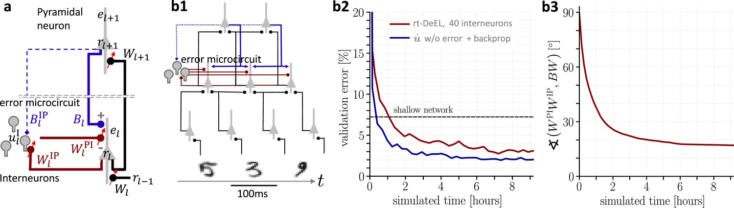
Hierarchical plastic microcircuits implement real-time dendritic error learning (rt-DeEL).
(a) Microcircuit with ‘top-down’ input (originating from peripheral motor activity, blue line) that is explained away by the lateral input via interneurons (dark red), with the remaining activity representing the error . Plastic connections are denoted with a small red arrow and nudging with a dashed line. (b1) Simulated network with 784-300-10 pyramidal-neurons and a population of 40 interneurons in the hidden layer used for the MNIST learning task where the handwritten digits have to be associated with the 10 fingers. (b2) Test errors for rt-DeEL with joint tabula rasa learning of the forward and lateral weights of the microcircuit. A similar performance is reached as with classical error backpropagation. For comparability, we also show the performance of a shallow network (dashed line). (b3) Angle derived from the Frobenius norm between the lateral pathway and the feedback pathway . During training, both pathways align to allow correct credit assignment throughout the network. Indices are dropped in the axis label for readability.
Appendix 1—figure 1
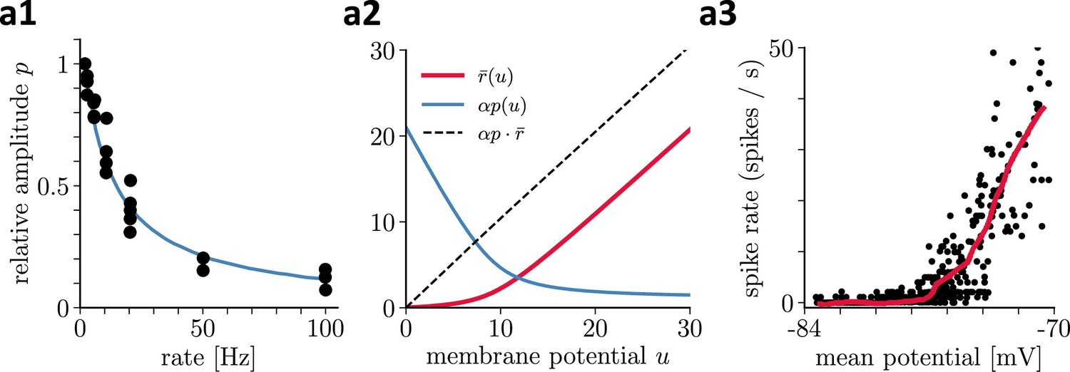
Recovering presynaptic potentials through short term depression.
(a1) Relative voltage response of a depressing cortical synapse recreated from Abbott et al., 1997, identified as synaptic release probability . (a2) The product of the low-pass filtered presynaptic firing rate times the synaptic release probability is proportional to the presynaptic membrane potential, . (a3) Average in vivo firing rate of a neuron in the visual cortex as a function of the somatic membrane potential recreated from Anderson et al., 2000, which can be qualitatively identified as the stationary rate derived in Equation 43.
Tables
Table 1
Mathematical symbols.
| Mathematical expression | Naming | Comment |
|---|---|---|
| Instantaneous (somatic) voltage | only for network neurons | |
| Instantaneous firing rate of neuron i | that looks linearly ahead in time | |
| Definition of low-pass filtering | See Equation 15 | |
| Low-pass filtered firing rate | postulated to be a function of | |
| Self-consistency eq. | for low-pass filtered rate | |
| Input rate vector, column | projects to selected neurons | |
| Low-pass filter input rates | instantaneously propagates | |
| Prospective error of neuroni | in apical dendrite | |
| Error of neuroni | in soma | |
| Mismatch energy in neuron i | between soma and basal dendrite | |
| Target voltage for output neuron o | could impose target on or | |
| Error of output neuron o | also called target error | |
| Cost contribution of output neuron o | between soma and basal dendrite | |
| Lagrangian | ||
| Discounted future voltage | prospective coordinates for NLA | |
| Self-consistency eq. | for discounted future voltage | |
| Neuronal Least Action (NLA) | expressed in prospect. coordinates | |
| Euler-Lagrange equations | turned into lookahead operator | |
| weights from input neurons | , most0 | |
| weights between network neurons | ||
| total weight matrix | ||
| instantaneous firing rate vector | column (indicated by transpose) | |
| Plasticity of | is a column, a row vector | |
| Target function formulated for | a functional of | |
| Func. implemented by forward network | instant. func. of , not | |
| Layers in forward network, w/o | Last-layer voltages: | |
| Weights from pyr to interneurons | lateral, within layer l | |
| Weights from inter- to pyr’neurons | lateral, within layer l | |
| Bottom-up weights from layerl–1 tol | between pyramidal neurons | |
| Top-down weights from layerl+1 tol | between pyramidal neurons | |
| Low-pass filtered apical error in layerl | top-down minus lateral feedback | |
| Somato-basal prediction error | is correct error for learning | |
| Interneuron mismatch energy | minimized to learn | |
| Apical mismatch energy | minimized to learn | |
| Learning rates for plasticity of… | … | |
| Hessian,. If pos. definite | ⇒ stable dynamics | |
| Corrected error | becomes 0 with | |
| Euler-Lagrange equations | satisfy | |
| Always the case after transient | exponentially decaying with | |
| Explicit diff. eq. | obtained by solving for | |
| Used to write the explicit diff. eq. | ||
| Used for contraction anaylsis, Equation 53 | ||
| Used to iteratively converge to | see Equation 46 | |
| Linear lookahead voltage | Latent Equilibrium, Appendix 4 |
Additional files
Download links
A two-part list of links to download the article, or parts of the article, in various formats.
Downloads (link to download the article as PDF)
Open citations (links to open the citations from this article in various online reference manager services)
Cite this article (links to download the citations from this article in formats compatible with various reference manager tools)
A neuronal least-action principle for real-time learning in cortical circuits
eLife 12:RP89674.
https://doi.org/10.7554/eLife.89674.3


