Robust, fast and accurate mapping of diffusional mean kurtosis
Figures
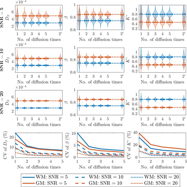
Simulation results on the effect of the number of diffusion times involved in the fitting of the sub-diffusion model (Equation 3) parameters and computing following (Equation 9) at various SNR levels.
The true values for (, , ) are set to (3 × 10⁻⁴, 0.75, 0.8125) to represent white matter (blue) and (5 × 10⁻⁴, 0.85, 0.4733) to represent grey matter (orange). Rows 1–3: Distributions of fitted parameter values using different number of diffusion times. 2′ represents an additional simulation using two diffusion times but set to be the same, so it has the same number of data points in the fitting as for using two different diffusion times. Row 4: Coefficient of variation (CV) of the parameter values fitted using different number of diffusion times.
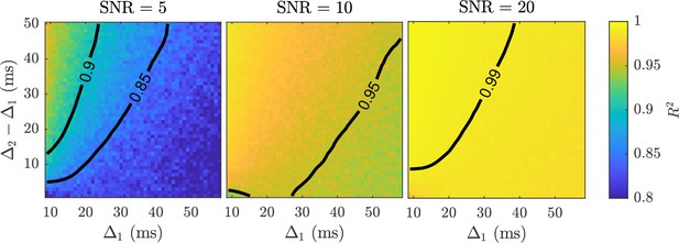
Surface plots of values achieved with fitting simulated data with two diffusion times, and , to the sub-diffusion model (Equation 3) at various SNR levels.
values were computed by comparing the estimated mean kurtosis with the true kurtosis. contours at the 0.85, 0.90, 0.95, and 0.99 levels have been provided for visualisation purposes.
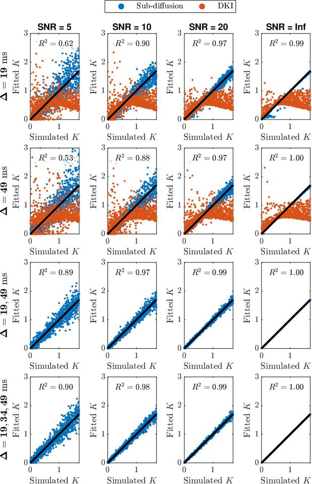
Scatter plots of simulated values versus fitted values for simulated data with different number of diffusion times at various SNR levels.
The simulated data is created using the sub-diffusion model with random normal noise (Equation 10). Blue dots represent kurtosis based on fitting the sub-diffusion model (Equation 3). Orange dots represent kurtosis based on fitting the traditional diffusional kurtosis imaging (DKI) model (Equation 6). Black line is a reference line for , indicating fitted kurtosis values are 100% matching the simulated ones.
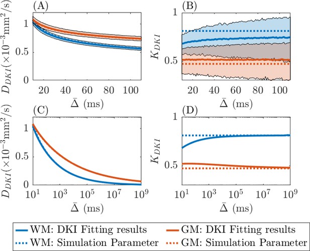
Time-dependence in diffusional kurtosis imaging (DKI) metrics using simulated data at different diffusion times ().
The true values for (, , ) used in the simulations are set to (3 × 10⁻⁴, 0.75, 0.8125) to represent white matter (blue dotted lines) and (5 × 10⁻⁴, 0.85, 0.4733) to represent grey matter (orange dotted lines). (A) and (B) use data with added random Gaussian noise (SNR = 20) to estimate the parameters and . (C) and (D) use noiseless data to obtain estimates for large values. Shaded regions in (A) and (B) represent the 95% confidence intervals of the estimates.
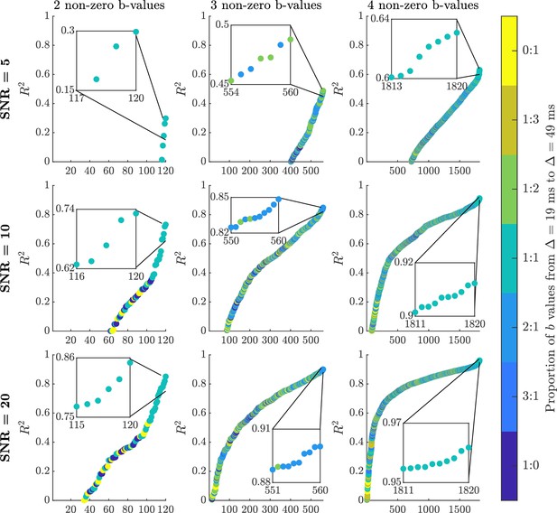
values for the b-value sampling optimisation based on DW-MRI data with SNR = 5, 10, and 20.
The specifically investigated b-value combinations using two, three, and four non-zero b-values have been ordered by the size of the value. The colour bar depicts the proportion of and b-values needed to produce the corresponding value. Note, the different b-value combinations were assigned a unique identifier, and these appear along the abscissa for each of the three non-zero b-value cases. The b-value combinations achieving the highest values are displayed in the inset pictures and the b-values are provided in Table 1.
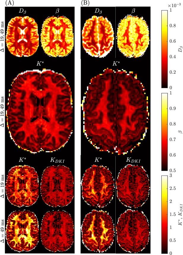
Spatially resolved maps of mean kurtosis shown for two example slices and two different subjects, Subject 3 rescan slice 71 (Panel A) and Subject 5 slice 74 (Panel B) from the Connectome 1.0 DW-MRI data.
Individual maps were generated using the sub-diffusion model framework (), as well as using the traditional approach (). The diffusion times, , used to generate each plot are provided for each case. We consider the mean kurtosis maps using two diffusion times as the benchmarks.
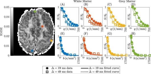
Representative error map and sample parameter fits for Subject 5 slice 74.
The DW-MRI data with two diffusion times was fitted to the sub-diffusion model in both q-space (A–D) and b-space (E–H), following (Equation 3) and (Equation 4), respectively. The first and second columns are voxels in white matter (30,20,74) and (45,56,74), respectively. The third and fourth columns are voxels in grey matter (58,35,74) and (34,78,74), respectively.
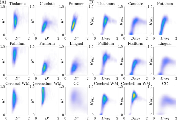
Distributions of the estimated parameter pair in different regions of the brain of all subjects, coloured by the probability density.
Yellow indicates high probability density, light blue indicates low probability density. Panel (A): distributions of , generated using the sub-diffusion model (Equation 3) with both . Panel (B): distributions of , generated using the standard diffusional kurtosis imaging (DKI) model (Equation 6) with . Kurtosis is dimensionless and diffusivity is in units of × 10–3 mm2/s.
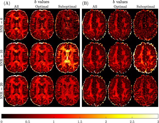
Spatially resolved maps of mean kurtosis shown for two example slices and two different subjects, Subject 3 rescan slice 71 (Panel A) and Subject 5 slice 74 (Panel B), based on SNR reduction of the Connectome 1.0 DW-MRI data.
Individual maps were generated using the sub-diffusion model framework (), considering optimal and sub-optimal four non-zero b-value sampling schemes. Here, two b-values with and two b-values with were selected for each case. The optimal b-values were chosen as the best for each SNR shown in Table 1. The sub-optimal b-values were chosen to have an = 0.3, 0.45, 0.5 to be about half of the maximum , for SNR = 6 (), SNR=10 (), and SNR = 20 (), respectively. The benchmark kurtosis map is provided in Figure 6.
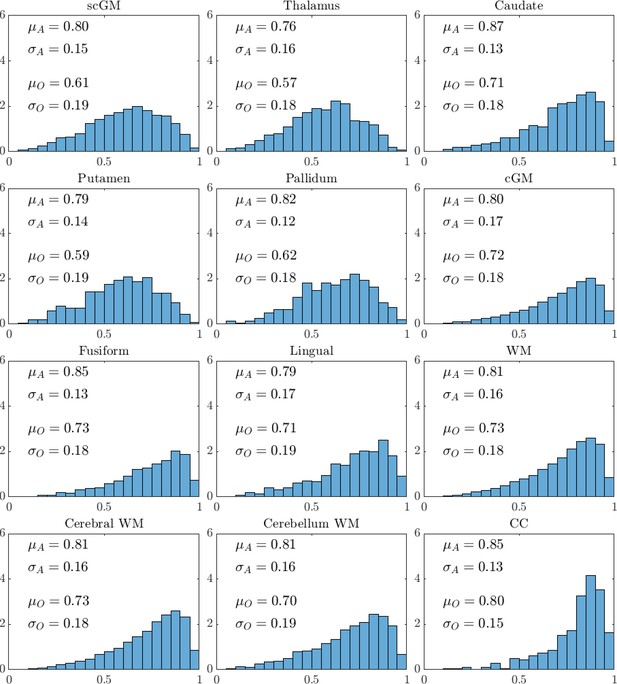
Interclass correlation coefficient (ICC) results for mean kurtosis are depicted for the 12 brain regions analysed.
The mean (μ) and standard deviation (σ) computed based on all the Connectome 1.0 DW-MRI data (subscript A), and the reduced data achieving an SNR = 10 with optimal four non-zero b-value sampling (subscript O), are provided for each brain region. Histograms were generated using all data. Mean kurtosis based on the optimised protocol was computed using the sub-diffusion framework using DW-MRI data with the four non-zero b-values suggested in Table 1 and diffusion encoding directions down sampled to achieve an SNR = 10.
Tables
A selection of the best b-value sampling regimes to achieve the highest value in the three cases considered.
The various categories correspond with two, three and four non-zero b-value sampling schemes, with and denoting the diffusion time setting used to generate the b-values. Note, entries are b-values in unit of s/mm2, and and were used to match the Connectome 1.0 DW-MRI data collection protocol. The entries listed at the bottom row are suggested optimal non-zero b-values for clinical practice.
| Two b-values | Three b-values | Four b-values | |||||||
|---|---|---|---|---|---|---|---|---|---|
| 350 | 6750 | 0.01 | 350, 800 | 2300 | 0.46 | 350, 4750 | 950, 4250 | 0.61 | |
| 800 | 2300 | 0.11 | 350 | 950, 4250 | 0.47 | 350, 6000 | 950, 6750 | 0.62 | |
| SNR = 5 | 350 | 4250 | 0.18 | 350 | 2300, 4250 | 0.47 | 350, 4750 | 950, 6750 | 0.62 |
| 350 | 950 | 0.26 | 50, 800 | 2300 | 0.48 | 350, 2400 | 950, 6750 | 0.63 | |
| 350 | 2300 | 0.30 | 350 | 950, 6750 | 0.49 | 350, 2400 | 950, 4250 | 0.63 | |
| 350 | 4250 | 0.63 | 350, 4750 | 2300 | 0.83 | 350, 2400 | 950, 9850 | 0.91 | |
| 800 | 4250 | 0.64 | 50, 800 | 2300 | 0.84 | 350, 3450 | 950, 6750 | 0.91 | |
| SNR = 10 | 350 | 950 | 0.67 | 350, 800 | 2300 | 0.84 | 350, 6000 | 950, 9850 | 0.91 |
| 350 | 2300 | 0.72 | 350, 1500 | 2300 | 0.84 | 350, 4750 | 950, 9850 | 0.91 | |
| 800 | 2300 | 0.73 | 350, 2400 | 2300 | 0.85 | 350, 3450 | 950, 9850 | 0.91 | |
| 1500 | 2300 | 0.77 | 350, 6000 | 2300 | 0.89 | 350, 4750 | 2300, 13,500 | 0.96 | |
| 350 | 950 | 0.78 | 50, 1500 | 4250 | 0.90 | 350, 4750 | 2300, 6750 | 0.96 | |
| SNR = 20 | 350 | 2300 | 0.80 | 350, 1500 | 2300 | 0.90 | 350, 6000 | 2300, 9850 | 0.96 |
| 800 | 4250 | 0.82 | 350, 4750 | 2300 | 0.90 | 350, 4750 | 2300, 9850 | 0.96 | |
| 800 | 2300 | 0.85 | 50, 2400 | 4250 | 0.90 | 350, 4750 | 950, 6750 | 0.96 | |
| 800 | 2300 | 0.85 | 350, 1500 | 2300 | 0.90 | 350, 1500 | 950, 4250 | 0.92 | |
Benchmark kurtosis values estimated using the Connectome 1.0 DW-MRI data for different regions of the human brain.
Results are provided for the traditional mean kurtosis () at two distinct diffusion times, and values () obtained based on fitting the sub-diffusion model across both diffusion times. Results are for grey matter (GM) and white matter (WM) brain regions, in categories of sub-cortical (sc) and cortical (c), and CC stands for corpus callosum. The pooled means and standard deviations across participants have been tabulated, along with the coefficient of variation in parentheses.
| scGM | 0.57 ± 0.23(40%) | 0.50 ± 0.24(48%) | 0.60 ± 0.21(35%) |
| Thalamus | 0.65 ± 0.19(30%) | 0.58 ± 0.22(39%) | 0.70 ± 0.17(25%) |
| Caudate | 0.41 ± 0.24(58%) | 0.37 ± 0.23(64%) | 0.39 ± 0.14(35%) |
| Putamen | 0.54 ± 0.21(40%) | 0.45 ± 0.22(49%) | 0.49 ± 0.13(27%) |
| Pallidum | 0.68 ± 0.25(37%) | 0.64 ± 0.26(41%) | 0.93 ± 0.18(19%) |
| cGM | 0.53 ± 0.24(46%) | 0.46 ± 0.23(51%) | 0.40 ± 0.16(39%) |
| Fusiform | 0.55 ± 0.22(40%) | 0.44 ± 0.22(49%) | 0.40 ± 0.15(37%) |
| Lingual | 0.59 ± 0.21(35%) | 0.53 ± 0.22(42%) | 0.47 ± 0.16(34%) |
| WM | 0.78 ± 0.20(25%) | 0.76 ± 0.19(26%) | 0.87 ± 0.22(25%) |
| Cerebral WM | 0.77 ± 0.19(25%) | 0.75 ± 0.19(26%) | 0.85 ± 0.22(26%) |
| Cerebellum WM | 0.99 ± 0.18(18%) | 0.95 ± 0.19(20%) | 1.07 ± 0.22(21%) |
| CC | 0.65 ± 0.22(35%) | 0.65 ± 0.22(34%) | 0.95 ± 0.25(26%) |
Benchmark values estimated using the Connectome 1.0 DW-MRI data for different regions of the human brain.
Results are provided for fitting the data at two distinct diffusion times, and fitting the sub-diffusion model across both diffusion times. Results are for grey matter (GM) and white matter (WM) brain regions, in categories of sub-cortical (sc) and cortical (c), and CC stands for corpus callosum. The pooled means and standard deviations across participants have been tabulated, along with the coefficient of variation in parentheses.
| scGM | 3.12 ± 0.96(31%) | 3.56 ± 1.03(29%) | 4.13 ± 0.86(21%) |
| Thalamus | 2.73 ± 0.83(30%) | 3.14 ± 0.89(28%) | 3.89 ± 0.81(21%) |
| Caudate | 4.32 ± 0.94(22%) | 4.80 ± 0.89(19%) | 5.21 ± 1.03(20%) |
| Putamen | 3.36 ± 0.58(17%) | 3.96 ± 0.54(14%) | 4.31 ± 0.44(10%) |
| Pallidum | 1.84 ± 0.63(34%) | 1.88 ± 0.67(36%) | 2.79 ± 0.52(19%) |
| cGM | 4.17 ± 0.97(23%) | 5.19 ± 0.96(19%) | 5.32 ± 0.90(17%) |
| Fusiform | 3.94 ± 0.83(21%) | 4.93 ± 0.74(15%) | 5.05 ± 0.69(14%) |
| Lingual | 3.78 ± 1.00(27%) | 4.62 ± 0.99(21%) | 5.01 ± 1.02(20%) |
| WM | 1.84 ± 0.79(43%) | 2.14 ± 0.93(43%) | 2.94 ± 0.72(24%) |
| Cerebral WM | 1.90 ± 0.77(41%) | 2.20 ± 0.92(42%) | 2.98 ± 0.71(24%) |
| Cerebellum WM | 0.81 ± 0.44(55%) | 1.17 ± 0.61(52%) | 2.03 ± 0.49(24%) |
| CC | 2.58 ± 1.84(71%) | 2.49 ± 1.91(76%) | 3.78 ± 2.12(56%) |
Benchmark β values estimated using the Connectome 1.0 DW-MRI data for different regions of the human brain.
Results are provided for fitting the data at two distinct diffusion times, and fitting the sub-diffusion model across both diffusion times. Results are for grey matter (GM) and white matter (WM) brain regions, in categories of sub-cortical (sc) and cortical (c), and CC stands for corpus callosum. The pooled means and standard deviations across participants have been tabulated, along with the coefficient of variation in parentheses.
| scGM | 0.74 ± 0.10(13%) | 0.69 ± 0.14(19%) | 0.81 ± 0.06(8%) |
| Thalamus | 0.70 ± 0.09(13%) | 0.63 ± 0.12(20%) | 0.78 ± 0.05(6%) |
| Caudate | 0.83 ± 0.07(8%) | 0.81 ± 0.07(9%) | 0.88 ± 0.04(5%) |
| Putamen | 0.79 ± 0.07(8%) | 0.77 ± 0.06(8%) | 0.85 ± 0.04(5%) |
| Pallidum | 0.61 ± 0.11(19%) | 0.47 ± 0.14(30%) | 0.72 ± 0.05(7%) |
| cGM | 0.81 ± 0.08(10%) | 0.83 ± 0.07(9%) | 0.87 ± 0.05(5%) |
| Fusiform | 0.81 ± 0.08(9%) | 0.83 ± 0.07(8%) | 0.87 ± 0.04(5%) |
| Lingual | 0.78 ± 0.09(11%) | 0.78 ± 0.09(12%) | 0.85 ± 0.05(6%) |
| WM | 0.61 ± 0.12(20%) | 0.52 ± 0.16(32%) | 0.74 ± 0.06(9%) |
| Cerebral WM | 0.62 ± 0.12(19%) | 0.53 ± 0.16(30%) | 0.74 ± 0.06(8%) |
| Cerebellum WM | 0.41 ± 0.16(39%) | 0.32 ± 0.19(60%) | 0.68 ± 0.06(9%) |
| CC | 0.61 ± 0.14(23%) | 0.43 ± 0.18(43%) | 0.71 ± 0.07(10%) |
Kurtosis values () under the optimal and sub-optimal b-value sampling regimes for specific brain regions.
was estimated based on fitting the sub-diffusion model to the Connectome 1.0 DW-MRI data with two diffusion times and selected four b-shells. Optimal b-value sampling is considered to have = 0.63, 0.91 and 0.96 for the SNR = 6, 10, and 20 columns, according to Table 1. Sub-optimal b-values are chosen to have = 0.3, 0.45, and 0.5, respectively, as reported in Figure 9. Individual entries are for grey matter (GM) and white matter (WM) brain regions, in categories of sub-cortical (sc) and cortical (c), and CC stands for corpus callosum. A reduction in SNR level was achieved by reducing the number of diffusion encoding directions in each b-shell of the DW-MRI data. The pooled means and standard deviations across participants have been tabulated, along with the coefficient of variation in parentheses. The entries identified in italic under the optimal b-value heading were found to be significantly different from the benchmark mean reported in Table 2. Sub-optimal result population means were mostly significantly different from the benchmark mean , and they are not italicised. The average errors (last column) are relative errors compared to the benchmark kurtosis values reported in Table 2.
| SNR = 6 | SNR = 10 | SNR = 20 | Average error for SNR = 6/10/20 | |
|---|---|---|---|---|
| Optimal b-values | ||||
| scGM | 0.47 ± 0.27(57%) | 0.65 ± 0.22(33%) | 0.61 ± 0.21(34%) | 37/23/12% |
| Thalamus | 0.57 ± 0.26(46%) | 0.75 ± 0.20(26%) | 0.71 ± 0.17(24%) | 33/20/11% |
| Caudate | 0.30 ± 0.20(68%) | 0.46 ± 0.17(38%) | 0.40 ± 0.15(38%) | 43/30/15% |
| Putamen | 0.38 ± 0.21(56%) | 0.58 ± 0.16(28%) | 0.52 ± 0.14(28%) | 40/28/13% |
| Pallidum | 0.66 ± 0.33(49%) | 0.90 ± 0.24(26%) | 0.89 ± 0.20(22%) | 39/19/12% |
| cGM | 0.40 ± 0.22(54%) | 0.51 ± 0.20(39%) | 0.45 ± 0.18(40%) | 30/36/19% |
| Fusiform | 0.37 ± 0.21(57%) | 0.54 ± 0.20(37%) | 0.45 ± 0.17(38%) | 35/43/20% |
| Lingual | 0.45 ± 0.22(50%) | 0.59 ± 0.19(33%) | 0.52 ± 0.18(34%) | 28/34/18% |
| WM | 0.72 ± 0.26(36%) | 0.91 ± 0.23(26%) | 0.89 ± 0.22(25%) | 23/13/8% |
| Cerebral WM | 0.71 ± 0.25(35%) | 0.89 ± 0.23(25%) | 0.88 ± 0.22(25%) | 22/13/8% |
| Sub-optimal b-values | ||||
| scGM | 0.31 ± 0.22(71%) | 0.82 ± 0.29(36) | 0.58 ± 0.25(43%) | 55/45/34% |
| Thalamus | 0.36 ± 0.23(65%) | 0.95 ± 0.25(27%) | 0.72 ± 0.19(26%) | 54/43/31% |
| Caudate | 0.23 ± 0.19(81%) | 0.57 ± 0.17(31%) | 0.40 ± 0.20(52%) | 56/57/40% |
| Putamen | 0.25 ± 0.16(67%) | 0.65 ± 0.17(26%) | 0.44 ± 0.20(46%) | 54/42/36% |
| Pallidum | 0.44 ± 0.29(66%) | 1.27 ± 0.32(25%) | 0.76 ± 0.25(33%) | 56/42/32% |
| cGM | 0.25 ± 0.17(67%) | 0.44 ± 0.14(33%) | 0.37 ± 0.17(47%) | 47/30/36% |
| Fusiform | 0.22 ± 0.15(68%) | 0.47 ± 0.16(35%) | 0.33 ± 0.17(52%) | 51/32/38% |
| Lingual | 0.29 ± 0.19(66%) | 0.53 ± 0.16(30%) | 0.39 ± 0.20(51%) | 48/29/40% |
| WM | 0.42 ± 0.18(44%) | 1.16 ± 0.36(31%) | 0.72 ± 0.22(31%) | 53/38/28% |
| Cerebral WM | 0.41 ± 0.18(43%) | 1.15 ± 0.35(31%) | 0.74 ± 0.20(28%) | 53/38/27% |
| Cerebellum WM | 0.47 ± 0.21(45%) | 1.27 ± 0.33(26%) | 0.35 ± 0.26(74%) | 57/24/72% |
| CC | 0.69 ± 0.42(61%) | 1.94 ± 0.44(23%) | 0.92 ± 0.19(20%) | 47/102/28% |
| Cerebellum WM | 0.83 ± 0.29(35%) | 1.17 ± 0.25(21%) | 1.15 ± 0.23(20%) | 27/15/11% |
| CC | 0.88 ± 0.36(41%) | 0.98 ± 0.31(31%) | 0.86 ± 0.25(29%) | 26/17/13% |


