Transformer-based spatial–temporal detection of apoptotic cell death in live-cell imaging
- Institute for Research in Biomedicine, Faculty of Biomedical Sciences, USI, Switzerland
- Department of Information Technology and Electrical Engineering, ETH Zurich, Switzerland
- Euler Institute, USI, Switzerland
- Institute of Cell Biology, University of Bern, Switzerland
- University of Manitoba, Canada
- Instituto de Biotecnología y Biomedicina (BioTecMed), Universitat de València, Spain
- Centro Nacional de Investigaciones Cardiovasculares, Spain
- Dalle Molle Institute for Artificial Intelligence, IDSIA, Switzerland
Figures
Figure 1 with 1 supplement
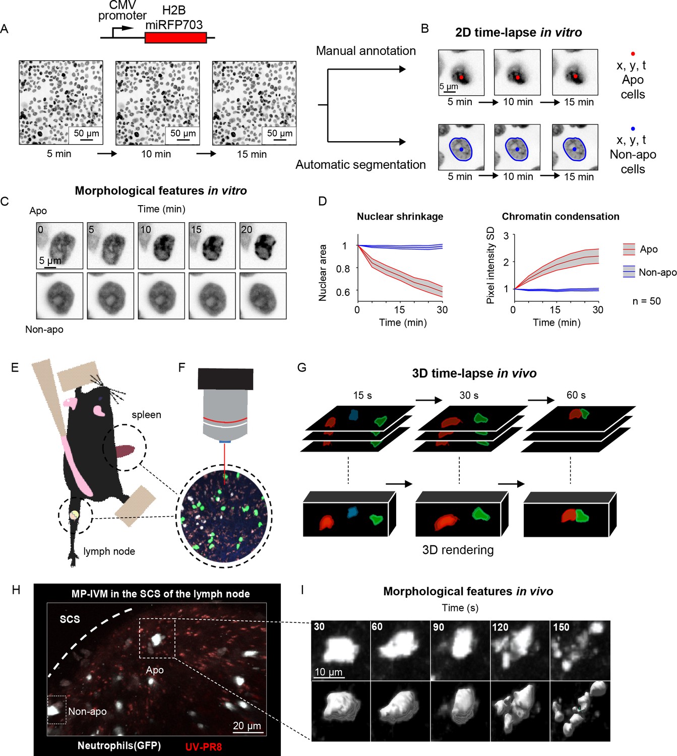
Generation of in vitro and in vivo live-cell imaging data.
(A) Micrographs depicting mammary epithelial MCF10A cells transduced with H2B-miRFP703 marker and grown to form a confluent monolayer. The monolayer was acquired with a fluorescence microscope for several hours with 1, 2, or 5 min time resolution. (B) The centroid (x, y) and the time (t) of apoptotic events were annotated manually based on morphological features associated with apoptosis. Nonapoptotic cells were identified by automatic segmentation of nuclei. (C) Image timelapses showing a prototypical apoptotic event (upper panels), with nuclear shrinkage and chromatin condensation, and a nonapoptotic event (bottom panels). (D) Charts showing the quantification of nuclear size (left) and the standard deviation (SD) of the nuclear pixel intensity (right) of apoptotic and nonapoptotic cells (n = 50). Central darker lines represent the mean, and gray shades bordered by light-colored lines represent the standard deviation. Nuclear area over time expressed as the ratio between areas at Tn and T0. (E) Simplified drawing showing the surgical setup for lymph node and spleen. (F, G) Organs are subsequently imaged with intravital two-photon microscopy (IV-2PM, F), generating 3D timelapses (G). (H) Representative IV-2PM micrograph and (I) selected crops showing GFP-expressing neutrophils (white) undergoing apoptosis. The apoptosis sequence is depicted by raw intensity signal (upper panels) and 3D surface reconstruction (bottom panels).
Figure 1—figure supplement 1
Generation of in vitro and in vivo microscopy data.
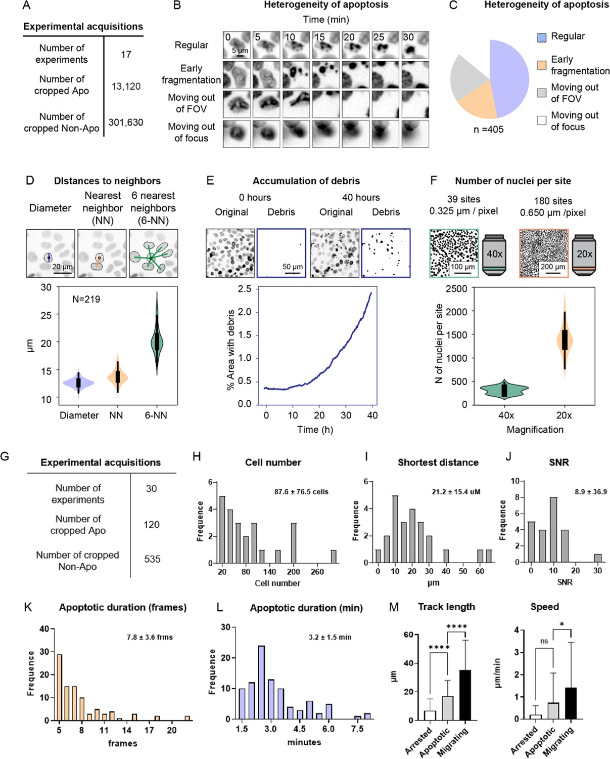
(A) Table reporting the number of entries of the dataset in vitro. (B) Timelapses showing the heterogeneity of the morphological appearance of apoptotic events. (C) Pie chart representing the frequency of the classes of morphological appearance in the entire dataset. (D) The density of the epithelium is quantified by comparing the diameter of the nuclei versus the distance to the nearest neighbor (NN), and to the six nearest neighbors (6-NN). Violin plot showing the mean of all cells of the first frame from (n = 219 field of views [FOVs]). (E) Data from a single FOV shows the accumulation of apoptotic debris over time, making the identification of newer apoptotic events difficult. In this experiment, MCF10A cells were treated with 1.25 µM doxorubicin for 40 hr. The image crops show the original nuclear channel and the binary images with identification of debris with a machine learning approach (Ilastik) and thresholding. The chart represents the area occupied by debris over time. (F) Two imaging modalities were used (40×, 20×), representative nuclear masks are shown in the left images. Violin plots show the mean number of nuclei in the first frame per FOV (40×: n = 39, 20×: n = 180). (G) Table reporting the number of entries of the dataset in vivo. (H–J) Quantification of cell numbers, shortest distance, and signal-to-noise ratio (SNR) in the generated intravital two-photon microscopy (IV-2PM) movies (n = 30). (K, L) Histograms representing the duration of the apoptotic events expressed in frames (K) and minutes (L). (M) Quantification of the track length (left) and cell speed (right) of apoptotic cells before disruption compared to arrested and migrating cells. Statistical comparison was performed with nonparametric Kruskal–Wallis test. Columns and error bars represent the mean and standard deviation, respectively. Significance is expressed as: *p≤0.05, **p≤0.01, ***p≤0.001, ****p≤0.0001.
Figure 2
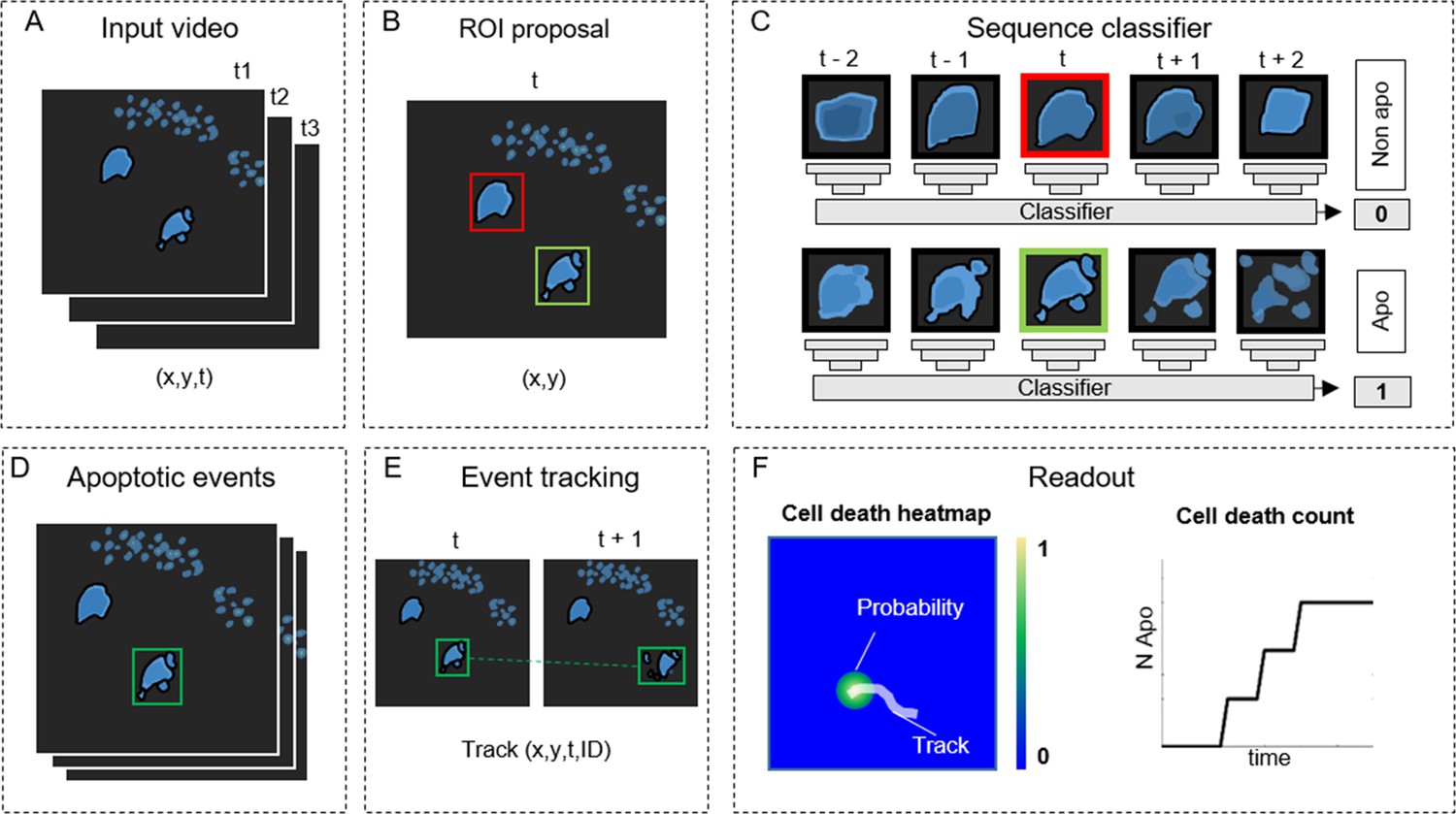
ADeS: a pipeline for apoptosis detection.
(A) ADeS input consists of single-channel 2D microscopy videos (x,y,t) (B) Each video frame is preprocessed to compute the candidate regions of interest (ROI) with a selective search algorithm. (C) Given the coordinates of the ROI at time t, ADeS extracts a series of snapshots ranging from t – n to t + n. A deep learning network classifies the sequence either as nonapoptotic (0) or apoptotic (1). (D) The predicted apoptotic events are labeled at each frame by a set of bounding boxes that (E) are successively linked in time with a tracking algorithm based on Euclidean distance. (F) The readout of ADeS consists of bounding boxes and associated probabilities, which can generate a probability map of apoptotic events over the course of the video (left) as well as providing the number of apoptotic events over time (right).
Figure 3
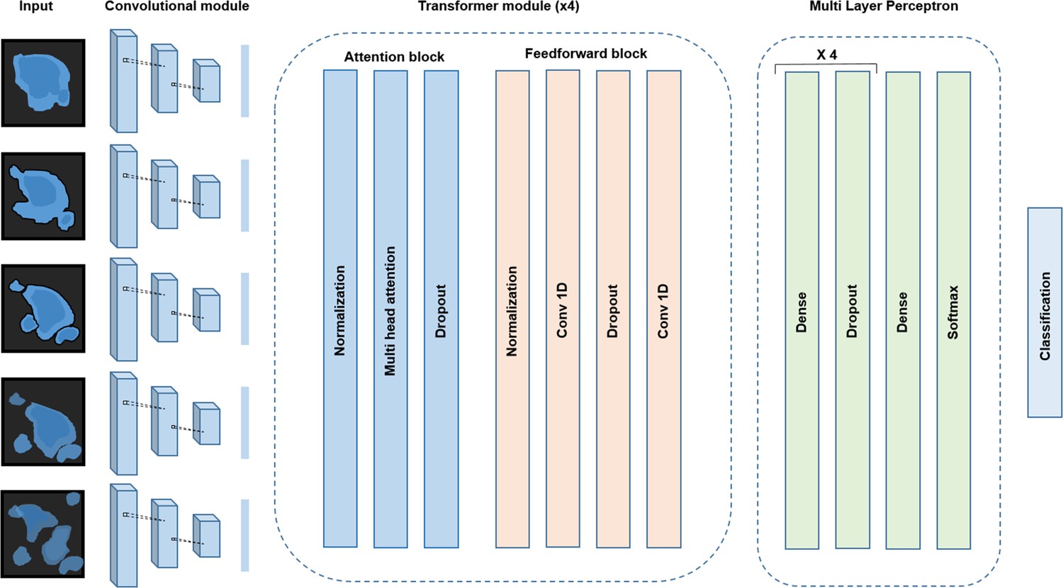
Conv-Transformer architecture at the core of ADeS.
Abstracted representation of the proposed Conv-Transformer classifier. The input sequence of frames is processed with warped convolutional layers, which extract the features of the images. The extracted features are passed into the four transformer modules, composed of attention and feedforward blocks. Finally, a multilayer perceptron enables classification between apoptotic and non-apoptotic sequences.
Figure 4 with 2 supplements
Training and performance in vitro.
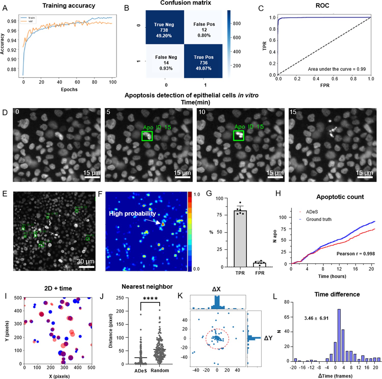
(A) Confusion matrix of the trained model at a decision-making threshold of 0.5. (B) Receiver-operating characteristic displaying the false positive rate (FPR) (specificity) corresponding to each true positive rate (TPR) (sensitivity). (C). Training accuracy of the final model after 100 epochs of training. (D) Representative example of apoptosis detection in a timelapse acquired in vitro (five replicates). (E) Multiple detection of nuclei undergoing apoptosis displays high sensitivity in densely packed field of views. (F) Heatmap representation depicting all apoptotic events in a movie and the respective probabilities. (G) Bar plots showing the TPR and FPR of ADeS applied to five testing movies, each one depicting an average of 98 apoptosis. (H) Time course showing the cumulative sum of ground-truth apoptosis (blue) and correct predictions (red). (I) 2D visualization of spatial–temporal coordinates of ground-truth (blue) and predicted apoptosis (red). In the 2D representation, the radius of the circles maps the temporal coordinates of the event. (J) Pixel distance between ADeS predictions and the nearest neighbor (NN) of the ground truth (left) in comparison with the NN distance obtained from a random distribution (right). The plot depicts all predictions of ADeS, including true positives and false positives. (K) Scatterplot of the spatial distance between ground truth and true positives of ADeS. Ground-truth points are centered on the X = 0 and Y = 0 coordinates. (L) Distribution of the temporal distance (frames) of the correct predictions from the respective ground-truth NN. Statistical comparison was performed with Mann–Whitney test. Columns and error bars represent the mean and standard deviation, respectively. Statistical significance is expressed as *p≤0.05, **p≤0.01, ***p≤0.001, ****p≤0.0001.
Figure 4—figure supplement 1
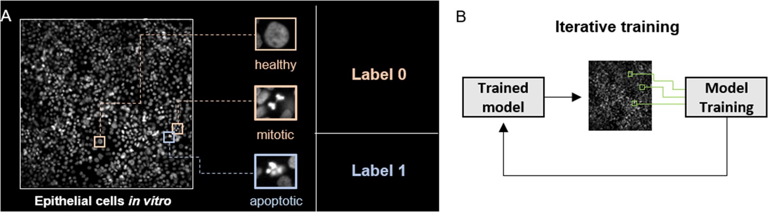
Training and performance in vitro.
(A) The training set describes a binary classification task in which the class label 1 contains the nuclei of epithelial cells undergoing apoptosis, while the class label 0 includes healthy and mitotic nuclei. (B) The class label 0 has been further expanded by iteratively including false positives generated by a trained network and applied to movies that contained no apoptotic events.
Figure 4—figure supplement 2
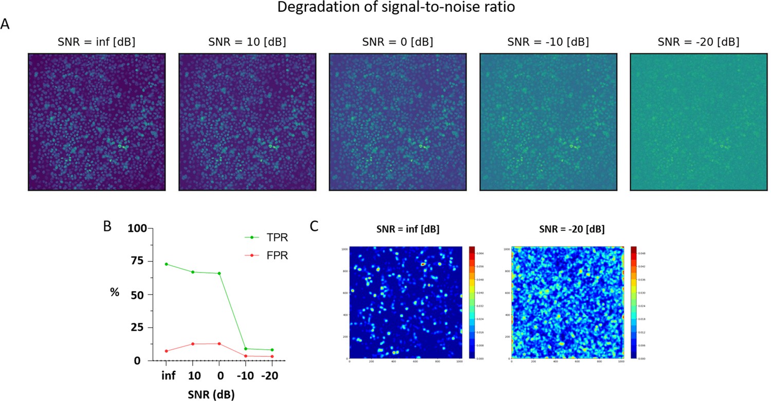
Effect of noise on ADeS performance.
(A) In vitro micrographs showing the same acquisition with the addition of different levels of noise measured in decibels (dB). High signal-to-noise ratio (SNR) values represent better video quality. (B) Plot showing the effect of increasing noise levels on the true positive rate (TPR) and false positive rate (TPR) of ADeS predictions (C) Noise effect visualized as a likelihood heatmaps. Higher noise generates frequent low-confidence predictions.
Figure 5
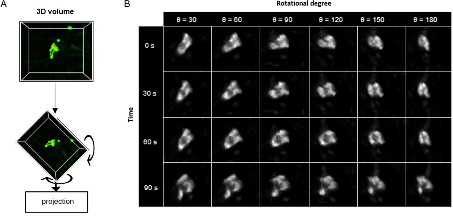
3D rotation of the in vivo dataset.
(A) Depiction of a 3D volume cropped around an apoptotic cell. Each collected apoptotic sequence underwent multiple 3D rotation in randomly sampled directions. The rotated 3D images were successively flattened in 2D. (B) Gallery showing the result of multiple volume rotations applied to the same apoptotic sequence. The vertical axis depicts the sequence over time, whereas the horizontal describes the rotational degree applied to the volumes.
Figure 6 with 1 supplement
Training and performance in vivo.
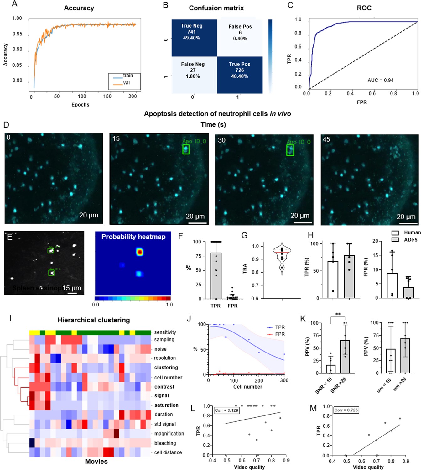
(A) Confusion matrix of the trained model at a decision-making threshold of 0.5. (B) Receiver-operating characteristic displaying the false positive rate (FPR) corresponding to each true positive rate (TPR). (C) Training accuracy of the final model trained for 200 epochs with data augmentations. (D) Image gallery showing ADeS classification to sequences with different disruption timing. The generated heatmap reaches peak activation (red) at the instant of cell disruption. (D) Representative snapshots of a neutrophil undergoing apoptosis. Green bounding boxes represents ADeS detection at the moment of cell disruption. (E) Representative micrograph depicting the detection of two eosinophils undergoing cell death in the spleen (left) and the respective probability heatmap (right). (F) ADeS performances expressed by means of TPR and FPR over a panel of 23 videos. (G) Tracking accuracy metric (TRA) measure distribution of the trajectories predicted by ADeS with respect to the annotated ground truth (n = 8) (H) Comparison between human and ADeS by means of TPR and FPR on a panel of five randomly sampled videos. (I) Hierarchical clustering of several video parameters producing two main dendrograms (n = 23). The first dendrogram includes videos with reduced sensitivity and is enriched in several parameters related to cell density and signal intensity. (J) Graph showing the effect of cell density on the performances expressed in terms of TPR and FPR (n = 13). (K) Comparison of the positive predictive value between videos with large and small signal-to-noise ratio (left) and videos with large and small shortest cell distance (right). (L, M) Selected video parameters are combined into a quality score that weakly correlates with the TPR in overall data (M, n = 23) and strongly correlates with the TPR in selected underperforming data (N, n = 8). Statistical comparison was performed with Mann–Whitney test. Columns and error bars represent the mean and standard deviation, respectively. Statistical significance is expressed as *p≤0.05, **p≤0.01, ***p≤0.001, ****p≤0.0001.
Figure 6—figure supplement 1
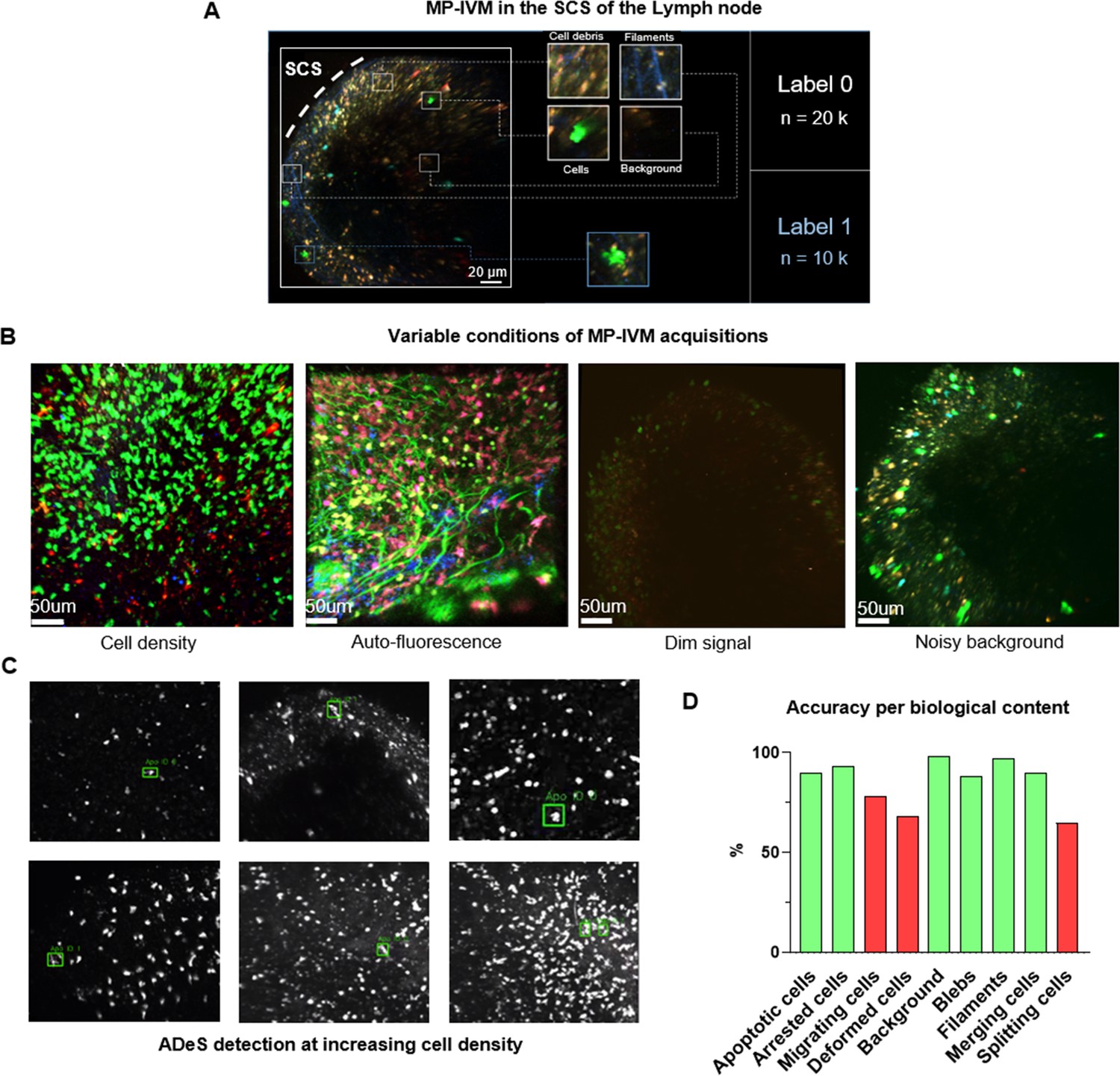
Training and deployment in vivo.
(A) The designed training set describes a binary classification task in which the class label 1 contains only apoptotic cells and the class label 0 encompasses all nonapoptotic content, including healthy cells, filaments, background, and cell debris. (B) Representative snapshots of variable and potentially challenging conditions in multiphoton intravital microscopy (MP-IVM), including high cell density, autofluorescence, dim signal, and noisy background. (C) Representative micrographs depicting the detection of apoptotic cells at increasing cell densities. (D) Graph showing the accuracy of ADeS in predicting the class label (0 or 1) of sequences containing different biological content. Red bars represent an accuracy below 80%.
Figure 7 with 1 supplement
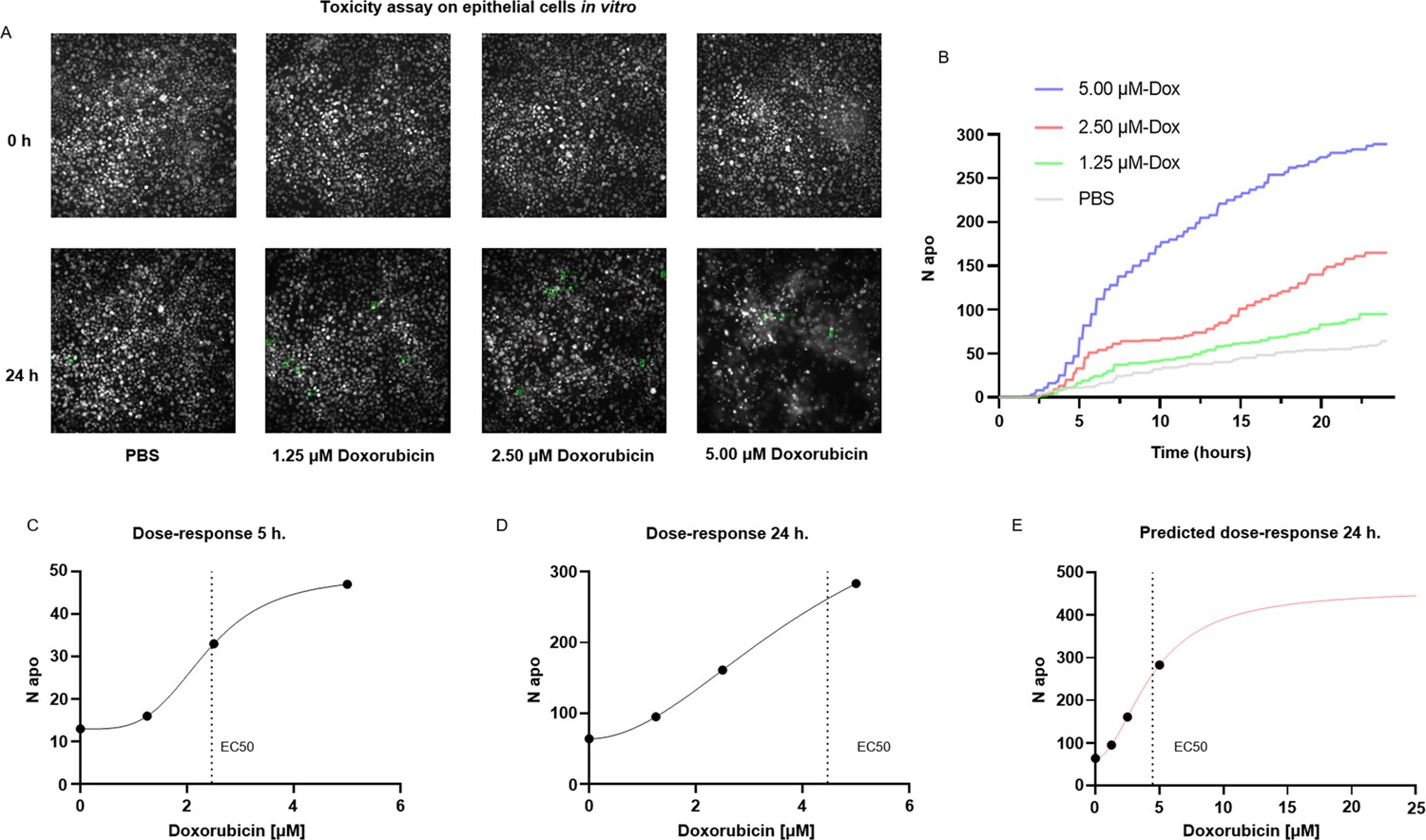
Applications for toxicity assay in vitro.
(A) Representative snapshots depicting epithelial cells in vitro at 0 and 24 hr after the addition of PBS and three increasing doses of doxorubicin, a chemotherapeutic drug and apoptotic inducer (three replicates). (B) Plot showing the number of apoptotic cells detected by ADeS over time for each experimental condition. (C, D) Dose–response curves generated from the drug concentrations and the respective apoptotic counts at 5 hr and 24 hr post-treatment. Vertical dashed lines indicate the EC50 concentration. (E) Dose–response curve projected from the fit obtained in (D). The predicted curve allows to estimate the response at higher drug concentrations than the tested ones.
Figure 7—figure supplement 1

Applications for toxicity assay in vitro.
(A) Schematic drawing representing in vitro-cultured T cells treated with staurosporine. (B) Confocal micrograph snapshot showing T cells at 60 min after treatment with staurosporine (left) compared to the untreated control group (right). (C) Survival assay plot of control (dotted lined) and treated samples (solid line) during the first 60 min post-treatment with staurosporine.
Figure 8
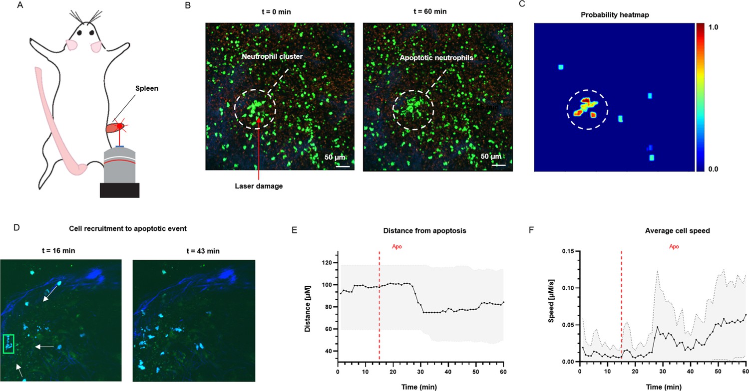
Measurement of tissue dynamics in vivo.
(A) Intravital two-photon micrographs showing ADeS detection of an apoptotic neutrophil (blue, left) and the subsequent recruitment of neighboring cells (right) in the popliteal LN at 19 hr following influenza vaccination. (B) Plot showing the distance of recruited neutrophils with respect to the apoptotic coordinates over time (n = 22). (C) Plot showing the instantaneous speed of recruited neutrophils over time (n = 22). The dashed vertical lines indicate the instant in which the apoptotic event occurs. Gray area defines the boundaries of maximum and minimum values. (D) Schematic drawing showing the intravital surgical setup of a murine spleen after inducing a local laser ablation. (E) Intravital two-photon micrographs showing the recruitment of GFP-expressing neutrophils (green) and the formation of a neutrophil cluster (red arrows) at 60 min after photo burning induction. (F) Application of ADeS to the generation of a spatiotemporal heatmap indicating the probability of encountering apoptotic events in the region affected by the laser damage. The dashed circle indicates a hot spot of apoptotic events.
Videos
Video 1
Prediction of apoptotic events in vitro.
Video 2
Prediction of apoptotic events in vivo.
Video 3
Noise affects the performance of ADeS in vivo.
Video 4
In vitro detections of apoptotic cells treated with PBS for 24h.
Video 5
In vitro detection of apoptotic cells treated with 1.25 μM doxorubicin.
Video 6
In vitro detection of apoptotic cells treated with 2.50 μM doxorubicin.
Video 7
In vitro detection of apoptotic cells treated with 5.00 μM doxorubicin.
Tables
Table 1
Comparison of deep learning architectures for apoptosis classification.
Comparative table reporting accuracy, F1, and AUC metrics for a CNN, 3DCNN, Conv-LSTM, and Conv-Transformer. The classification accuracy is reported for static frames or image sequences. The last column shows which cell death study employed the same baseline architecture displayed in the table.
| Classifier architecture | Frame accuracy | Sequence accuracy | F1 | AUC | Study |
|---|---|---|---|---|---|
| CNN | 74% ± 1.3 | NA | 0.77 | 0.779 | La Greca et al., 2021; Verduijn et al., 2021 |
| 3DCNN | NA | 91.22 % ± 0.15 | 0.91 | 0.924 | - |
| Conv-LSTM | NA | 97.42% ± 0.09 | 0.97 | 0.994 | Kabir et al., 2022; Mobiny et al., 2020 |
| Conv-Transformer | NA | 98.27% ± 0.25 | 0.98 | 0.997 | Our |
-
CNN, convolutional neural network; NA, nonapplicable.
Table 2
Comparison of cell death identification studies.
Table reporting all studies on cell death classification based on machine learning. For each study, we included the reported classification accuracy, the experimental conditions of the studies, the target input of the classifier, and the capability of performing detection on static frames or microscopy timelapses. Met conditions are indicated with a green check. Moreover, for each study we reported the architecture of the classifier and the number of apoptotic cells in the training set. NA stands for not available and indicates that the information is not reported in the study.
| Study | Input of the classifier | Reported classification accuracy | In vitro | In vivo | DetectionIn frame | Detection in movies | Classifier architecture | N cell death |
|---|---|---|---|---|---|---|---|---|
| Our | Frame sequence | 98.27% | ✓ | ✓ | ✓ | ✓ | Conv-Transformer | 13,120 |
| Jin et al., 2022 | Frame | 93% | ✓ | ✘ | ✘ | ✘ | Logistic regression | NA |
| Verduijn et al., 2021 | Frame | 87% | ✓ | ✘ | ✘ | ✘ | VGG-19 | 19,339 |
| Kabir et al., 2022 | Frame sequence | 93% | ✓ | ✘ | ✘ | ✘ | ResNet101-LSTM | 3172 |
| La Greca et al., 2021 | Frame | 96.58% | ✓ | ✘ | ✘ | ✘ | ResNet50 | 11,036 |
| Mobiny et al., 2020 | Frame sequence | 93.8% | ✓ | ✘ | ✘ | ✘ | CapsNet-LSTM | 41,000 |
| Kranich et al., 2020 | Frame | 93.2% | ✓ | ✘ | ✘ | ✘ | CAE-RandomForest | 27,224 |
| Vicar et al., 2020 | Frame sequence | NA | ✓ | ✘ | ✓ | ✓ | biLSTM | 1745 |
| Jimenez-Carretero et al., 2018 | Frame | NA | ✓ | ✘ | ✓ | ✘ | R-CNN | 255,215 |
Additional files
Download links
A two-part list of links to download the article, or parts of the article, in various formats.
Downloads (link to download the article as PDF)
Open citations (links to open the citations from this article in various online reference manager services)
Cite this article (links to download the citations from this article in formats compatible with various reference manager tools)
Transformer-based spatial–temporal detection of apoptotic cell death in live-cell imaging
eLife 12:RP90502.
https://doi.org/10.7554/eLife.90502.3


