Deciphering the chemical language of inbred and wild mouse conspecific scents
- Department of Chemosensation, Institute for Biology II, RWTH Aachen University, Germany
- Department of Medical Neurobiology, Institute for Medical Research Israel Canada, Faculty of Medicine, The Hebrew University of Jerusalem, Israel
- Institute of Neurophysiology, Uniklinik RWTH Aachen University, Germany
- Research Training Group 2416 MultiSenses – MultiScales, RWTH Aachen University, Germany
- BIOCEV group, Department of Zoology, Faculty of Science, Charles University, Czech Republic
Figures
Figure 1 with 1 supplement
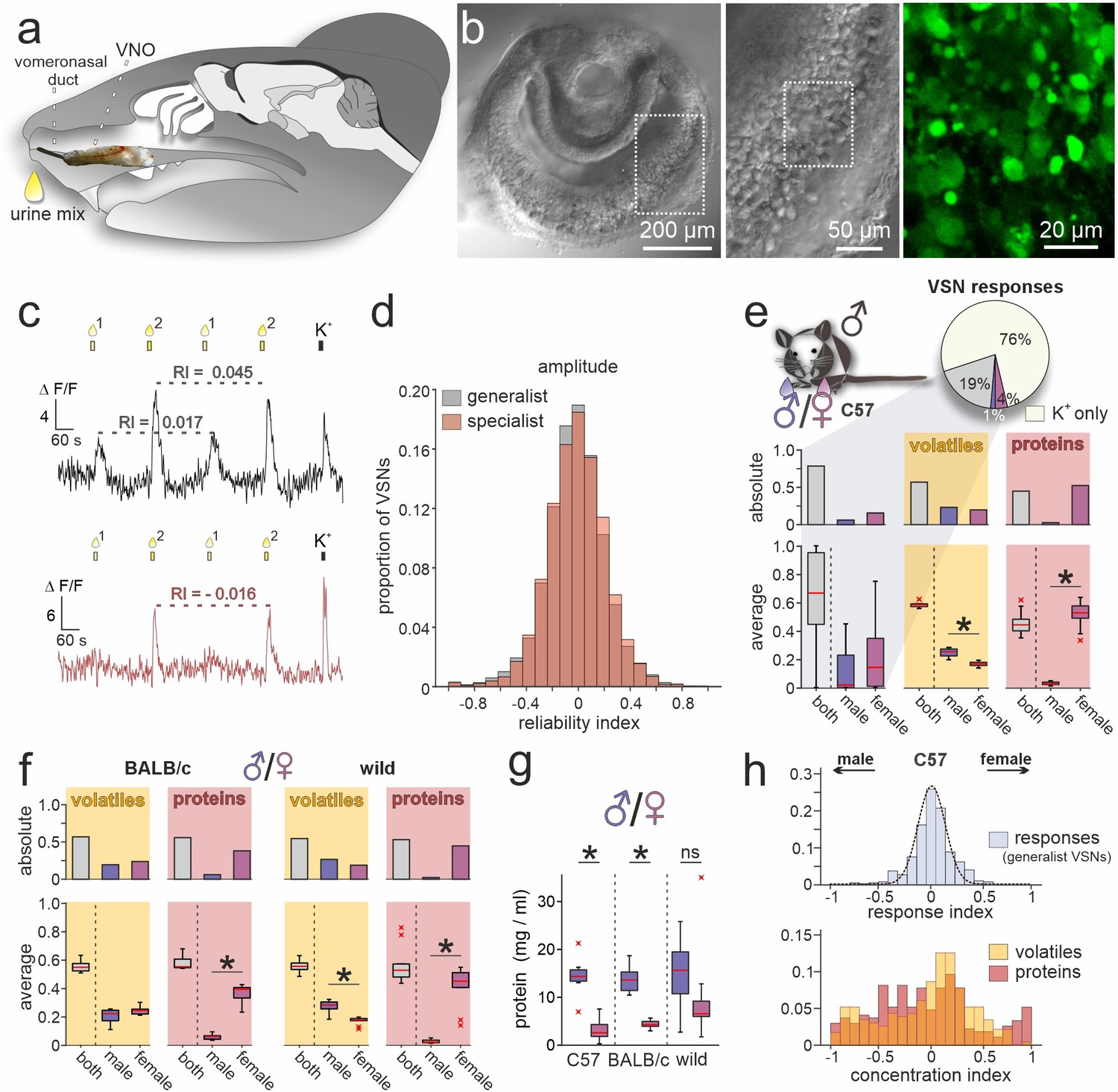
A population activity assay captures sex-dependent stimuli representations.
(a) Anatomical location of the rodent vomeronasal organ (VNO). Schematic depicting a sagittal section through a mouse head with an overlay of a VNO image. The vomeronasal duct that opens into the anterior nasal cavity is also highlighted. (b) Overview (left) and zoomed-in (middle) differential interference contrast micrograph showing an acute coronal VNO section from an adult C57BL/6 mouse. Confocal fluorescence image (right; dashed rectangle in middle) depicting a depolarization (elevated K+) dependent cytosolic Ca2+ increase in vomeronasal sensory neuron (VSN) somata after bulk loading with Cal-520 AM. (c) Original traces showing changes in cytosolic Ca2+ concentration over time in two representative VSN somata. VNO slices were briefly challenged with two mixtures of diluted mouse urine (1:100; 10 s; top yellow bars/droplets). Repeated stimulation in alternating sequence at 180 s inter-stimulus intervals (Wong et al., 2018) was followed by membrane depolarization upon exposure to elevated extracellular K+ (50 mM; 10 s). According to individual response type, VSNs were categorized as ‘generalists’ (top) or ‘specialists’ (bottom). Signal amplitudes in response to the same stimulus allowed calculation of a reliability index (RI) as a measure of signal robustness. (d) Amplitude reliability index histograms of all generalist VSNs (gray; n=10,258) and all specialist VSNs (red; n=6457) recorded in this study. Note that for both response types, indices are normally distributed with a narrow central peak around zero. (e) Quantification of results obtained from recordings in VSNs from male C57BL/6 mice challenged with male versus female C57BL/6 urine stimuli. Pie chart (top) illustrates the proportions of generalist (19%) and specialist neurons (1% and 4%, respectively) among all K+-sensitive VSNs (n=1999). Bar graph (middle, left) breaks down the summed total of urine-sensitive neurons by categories and compares their distribution with the proportions of volatile organic compounds (VOCs) (yellow background; n=405) and proteins (red background; n=601) found either in both male and female urine (gray bars) or exclusively in samples from one sex (male, dark blue; female, purple). Box-and-whisker plots (bottom, left) illustrating generalists-to-specialists ratios over individual experiments (n=19). Boxes represent the first-to-third quartiles. Whiskers represent the 10th and 90th percentiles, respectively. Outliers (1.5 IQR; red x) are plotted individually. The central red band represents the population median (P0.5). Results are shown in relation to box-and-whisker plots that outline chemical content data obtained from paired comparisons (n=10 individuals per group). (f) Molecular composition of male versus female urine from BALB/c and wild mice. Bar graphs (top) display proportions of VOCs (yellow background; BALB/c, n=514; wild, n=462) and proteins (red background; BALB/c, n=407; wild, n=526) found either in both male and female urine (gray bars) or exclusively in samples from one sex (male, dark blue; female, purple). Box-and-whisker plots (bottom) quantify category ratios for individual paired experiments (n=10 individuals per group). (g) Quantification (Bradford assay) of protein/peptide content in urine samples from C57BL/6, BALB/c, and wild mice, respectively (n=10 each). Note the substantially increased protein content in male samples. (h) Response index histogram (top) obtained from generalist C57BL/6 VSNs that responded to both male and female same-strain urine (data corresponding to (e)). Fitted Gaussian curve (dashed line) centers close to zero (peak = –0.03) and shows a relatively narrow width (σ=0.13). By contrast, concentration index histograms (bottom), calculated for VOCs (yellow) and proteins (red) found in both male and female urine samples, are heterogeneous and not normally distributed. Asterisks (*) indicate statistical significance, p<0.05; Wilcoxon signed-rank test (for VSN functional data), Mann-Whitney U test (for molecular profiling), and unpaired t-test (for protein content comparison shown in (g)).
Figure 1—figure supplement 1
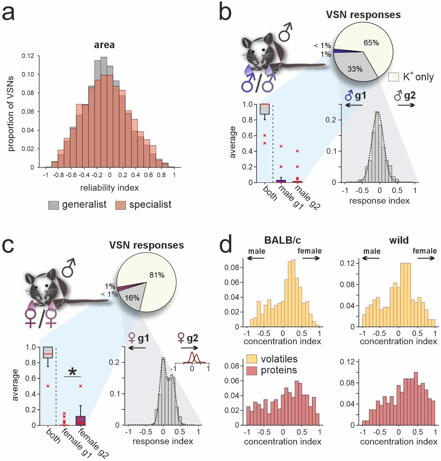
A VSN population activity assay with a low level of biological and experimental noise.
(a) Area under curve response reliability index histograms of all generalist vomeronasal sensory neurons (VSNs) (gray; n=10,258) and all specialist VSNs (red; n=6457) recorded from in this study. Note that for both response types, indices are normally distributed. While histograms peak around zero, distributions are much broader as compared to amplitude-based reliability index histograms (Figure 1d). (b and c) Quantification of VSN responses recorded from male C57BL/6 mice challenged with urine stimuli from two different male C57BL/6 mouse cohorts (b) or two different female C57BL/6 mouse cohorts (c). Pie charts (top) illustrate the proportions of generalist (gray; 33% (b) and 16% (c), respectively) and specialist neurons (≤1%; dark versus light blue (b) and dark versus light red (c), respectively) among all K+-sensitive VSNs (n=1867 (b) and n=1946 (c), respectively). Box-and-whisker plots (bottom, left) break down the urine-sensitive neurons by categories and illustrate the generalists-to-specialists ratios over individual experiments (n=21). Boxes represent the first-to-third quartiles. Whiskers represent the 10th and 90th percentiles, respectively. Outliers (1.5 IQR; red x) are plotted individually. The central red band represents the population median (P0.5). Response index histograms (bottom, left) depict signal amplitude strength distributions from generalist VSNs that responded to both paired stimuli (i.e., cohort/group 1 [g1] and cohort/group 2 [g2]). Multi-peak fitting with Gaussian curves (dashed lines) resulted either in a narrow single Gaussian that centers close to zero (b; peak = –0.06, σ=0.16) or two additive Gaussian curves that best represented the calculated index distribution (c; peak 1=–0.01, peak 2=0.25). Asterisk (*) indicates statistical significance, p<0.05; Wilcoxon signed-rank test. (d) Concentration index histograms that outline individual compound concentration imbalances of volatile organic compounds (VOCs) (yellow; top) and proteins (red; bottom) that are found in both male and female urine samples of either BALB/c (left) or wild (right) mice. Histograms are heterogeneous and data are not normally distributed.
Figure 2 with 3 supplements
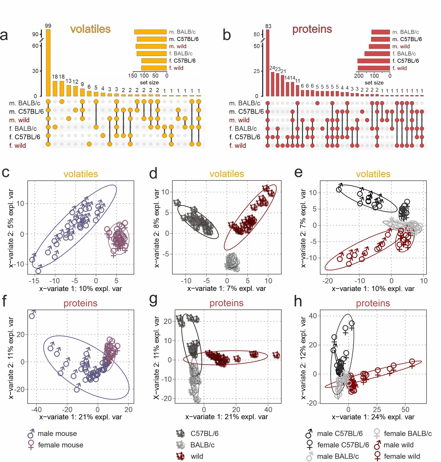
Chemical profiling of urine content identifies unique sex- and strain-specific molecular fingerprints.
(a, b) Matrix layout for all intersections of volatile organic compounds (VOCs) (a) and proteins (b) among the six sex/strain combinations, sorted by size. Colored circles in the matrix indicate combinations that are part of the intersection. Bars above the matrix columns represent the number of compounds in each intersection. Empty intersections have been removed to save space. Horizontal bar charts (bottom, left) depict the number of VOCs (a) and proteins (b) detected in each urine set. Proteomics data are available via ProteomeXchange with identifier PXD042324. (c–h) Sparse partial least-squares discriminant analysis (sPLS-DA) score plots depicting the first two sPLS-DA components, which explain 7–10% (1st component) and 5–8% (2nd component) of VOC data variance (c–e) as well as 21–24% (1st component) and 11–12% (2nd component) of protein data variance (f–h), respectively. Ellipses represent 95% confidence intervals. Plots demonstrate sample clustering according to the urine donors’ sex (c, f), genetic background (d, g), or sex/strain combination (e, h). Each data point represents a sample from an individual animal (n=60; 10 samples per sex/strain combination), with sample type colored according to symbol legend (bottom).
Figure 2—figure supplement 1
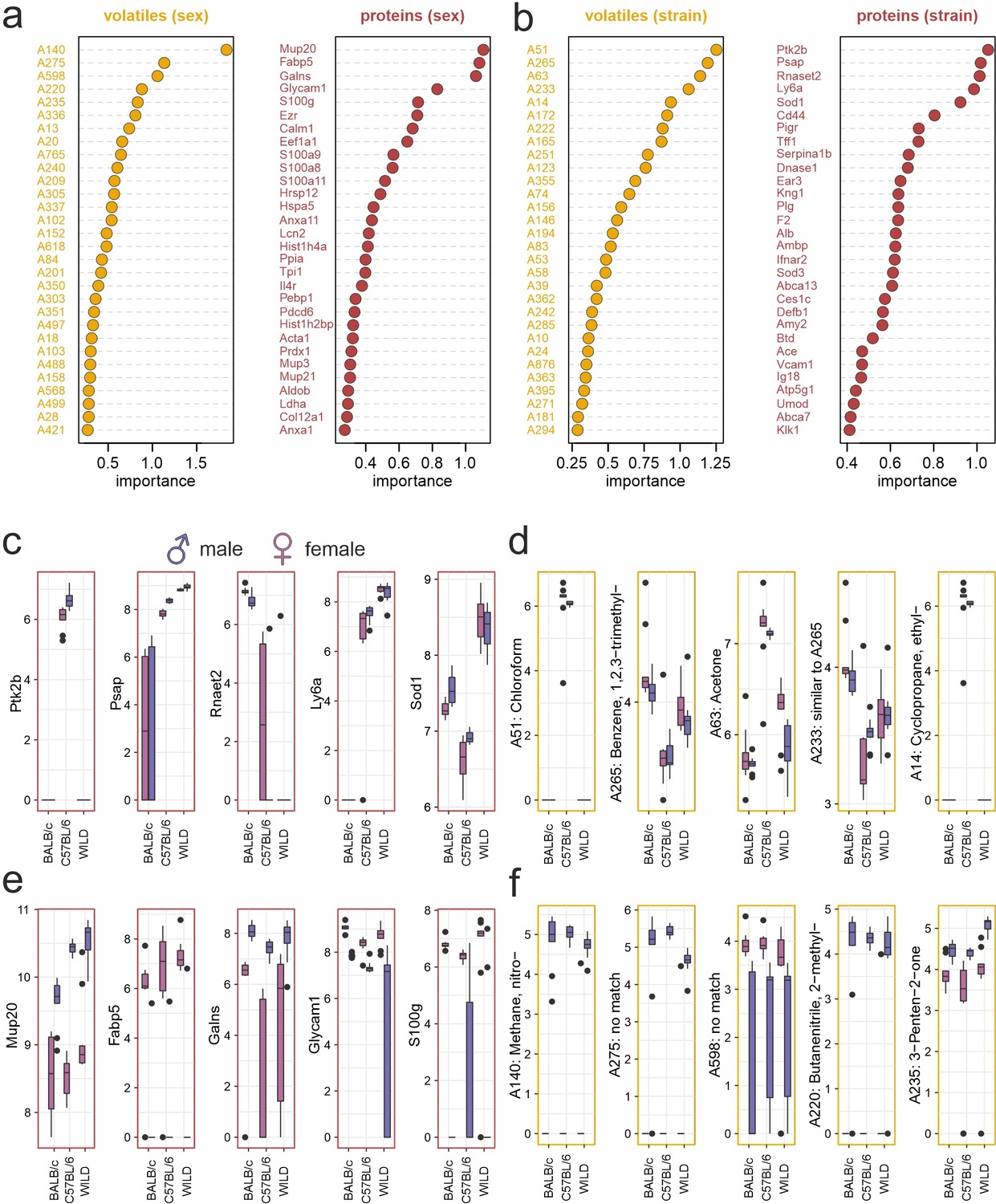
The most informative VOCs and proteins that discriminate sex and strain, respectively.
(a, b) After training Random Forest classifiers (Breiman, 2001), lists of ‘Gini importance’ (Breiman, 2001) scores rank urine volatile organic compounds (VOCs) (a; yellow) and proteins (b; red) that are likely most informative to decode sex and strain, respectively. (c–f) Box-and-whisker plots quantify concentrations of the respective five VOCs (c, e) and proteins (d, f) that are ranked most important/informative (a, b). Data are plotted as log2 signal intensity for each of the six sex/strain combinations (10 individual samples each). Red (female) and blue (male) boxes represent sex; strain as indicated. Boxes represent the first-to-third quartiles. Whiskers represent the 10th and 90th percentiles, respectively. Outliers (1.5 IQR; black dots) are plotted individually. Central bands represent the population median (P0.5).
Figure 2—figure supplement 2
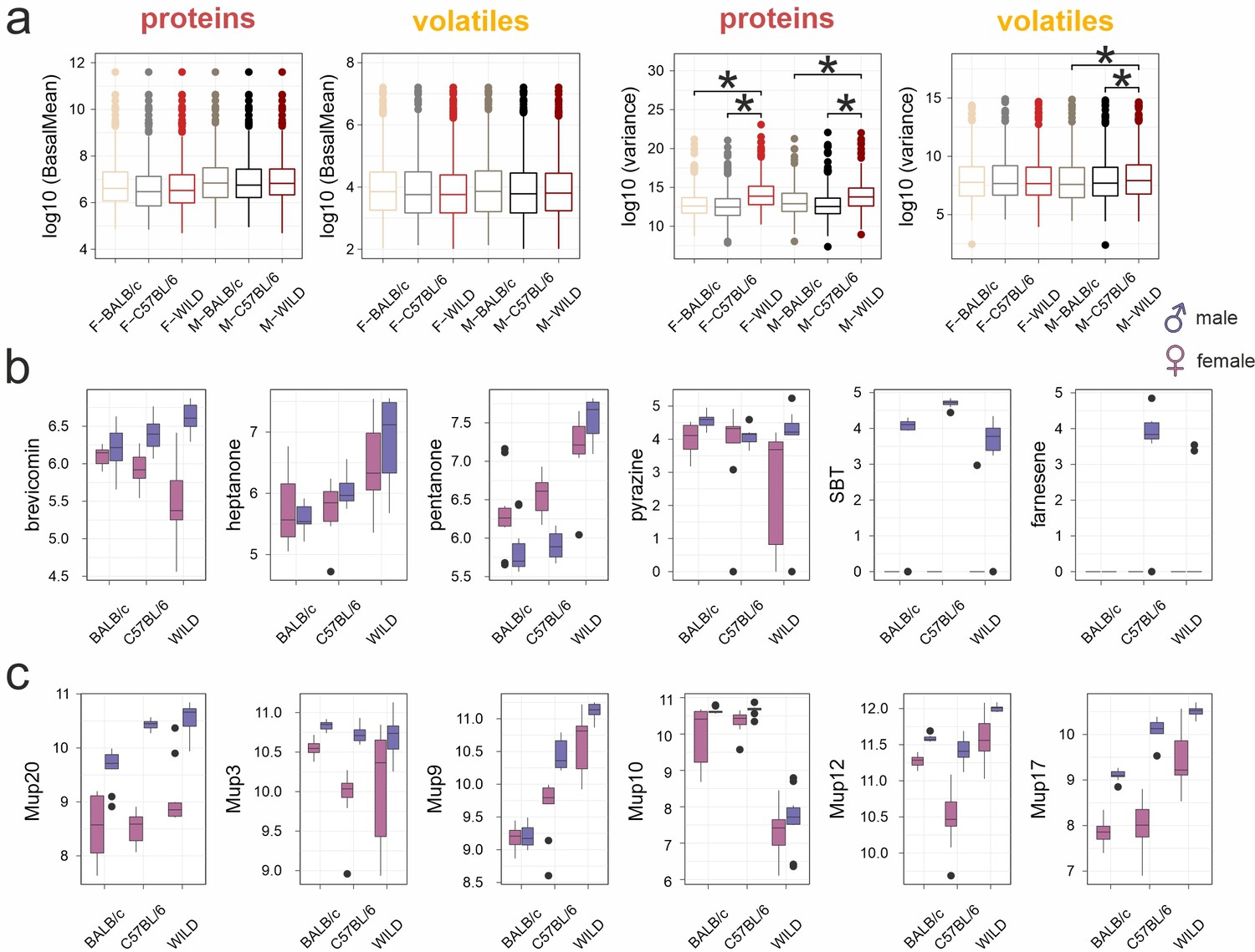
Protein and VOC content in mouse urine across strains.
(a) Box-and-whisker plots illustrating mean protein and volatile organic compound (VOC) content (left) as well as individual compound concentration variance (right) for the six sex/strain combinations (10 individual samples each). Asterisks (*) indicate statistical significance, p<0.05, Kruskal-Wallis test. (b, c) Box-and-whisker plots quantify concentrations of previously reported VOC (b) and major urinary protein (Mup) (c) semiochemicals, respectively. Data are plotted as log2 signal intensity for each of the six sex/strain combinations (10 individual samples each). Red (female) and blue (male) boxes represent sex; strain as indicated. Boxes depict the first-to-third quartiles. Whiskers represent the 10th and 90th percentiles, respectively. Outliers (1.5 IQR; black dots) are plotted individually. Central bands represent the population median (P0.5).
Figure 2—figure supplement 3
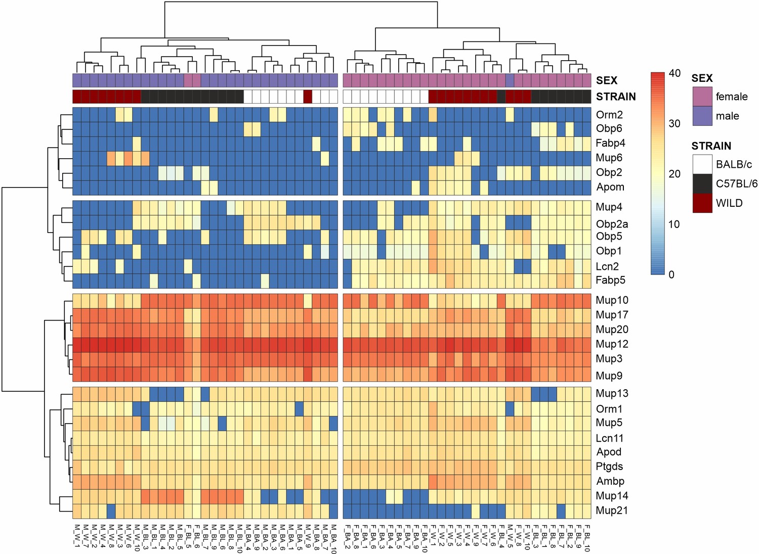
Hierarchical clustering of mouse urine lipocalin content reveals an unexpectedly diverse repertoire of 27 lipocalins.
The horizontal tree clusters lipocalins according to proteomic homology based on similarities in protein abundances. The vertical tree clusters the 60 individual urine samples (10 samples for each of the 6 sex/strain combinations) according to patterns of lipocalin abundance (pseudocolors).
Figure 3
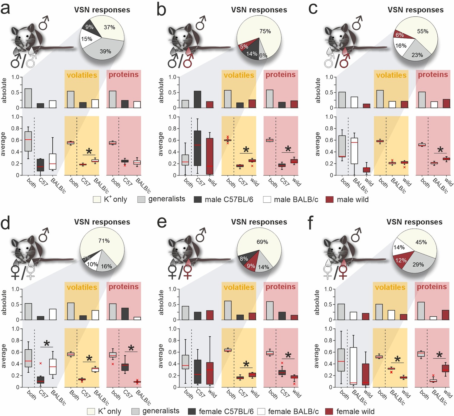
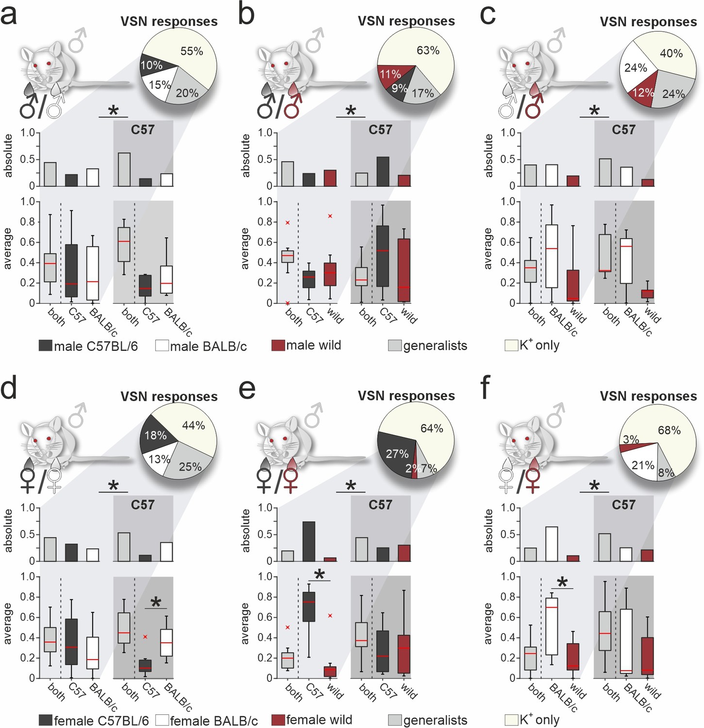
Selective vomeronasal sensory neuron (VSN) response profiles upon stimulation with strain-specific signatures.
Quantitative comparison between VSN responses to paired stimuli and their respective chemical signatures. Neurons of male C57BL/6 mice were challenged with male (a–c) or female (d–f) urine, respectively. Response profiles are compared upon stimulation with C57BL/6 versus BALB/c urine (a and d), C57BL/6 versus wild stimuli (b and e), and BALB/c versus wild urine (c and f), respectively. Pie charts (top) illustrate the proportions of generalist (light gray) and specialist neurons (dark gray, white, and purple, respectively) among all K+-sensitive VSNs (a, n=1855; b, n=4116; c, n=2462; d, n=2376; e, n=3230; f, n=3377). Bar graphs (left) break down the urine-sensitive neurons by categories and compare their distribution with the proportions of volatile organic compounds (VOCs) (middle; yellow background; a, n=450; b, n=448; c, n=479; d, n=480; e, n=405; f, n=492) and proteins (right; red background; a, n=317; b, n=330; c, n=334; d, n=657; e, n=715; f, n=584) found either in both urine types (gray bars) or exclusively in samples from one group (color code as in pie charts). Box-and-whisker plots (bottom) illustrate generalist-to-specialist VSN category ratios over individual experiments (a, n=6; b, n=10; c, n=7; d, n=9; e, n=10; f, n=12). Boxes represent the first-to-third quartiles. Whiskers represent the 10th and 90th percentiles, respectively. Outliers (1.5 IQR; red x) are plotted individually. The central red band represents the population median (P0.5). Results are shown in relation to box-and-whisker plots that outline chemical content data obtained from paired comparisons (n=10 individuals per group). Asterisks (*) indicate statistical significance, p<0.05, Wilcoxon signed-rank test.
Figure 4
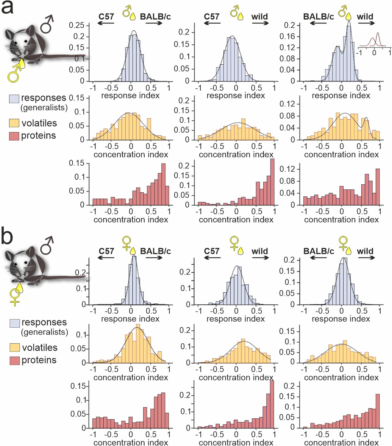
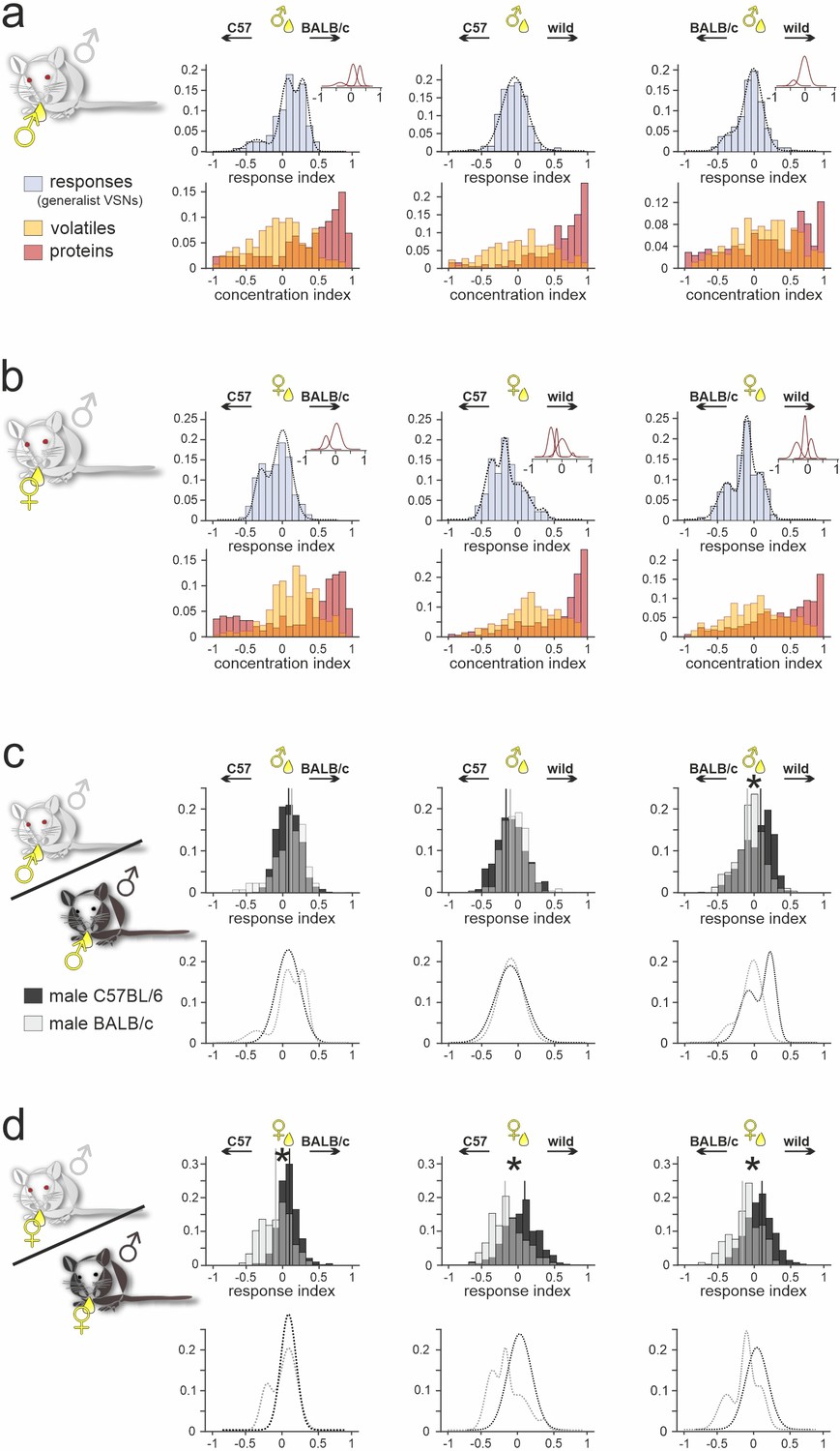
Strain-dependent concentration imbalances exert relatively mild effects on vomeronasal sensory neuron (VSN) population response homogeneity.
Comparison of male C57BL/6 generalist VSN response preferences, upon stimulation with paired urine stimuli from different strains, with strain-dependent concentration imbalances among volatile organic compounds (VOCs) and proteins, respectively. (a, b) Response index histograms (top rows) depict distributions of generalist data outlined in Figure 3 (gray bars). With one exception (a (right), male BALB/c versus male wild), histograms are well fitted by single Gaussian curves (dashed lines) that each center relatively close to zero (a (left), peak = 0.08, σ=0.18; a (middle), peak = –0.11, σ=0.21; a (right), 1st peak = –0.12, 1st σ=0.14; 2nd peak = 0.21, 2nd σ=0.09; b (left), peak = 0.07, σ=0.12; b (middle), peak = 0.03, σ=0.23; b (right), peak = 0.05, σ=0.18). Concentration index histograms (middle and bottom rows), calculated for VOCs (yellow) and proteins (red) found in both tested urine samples, are more heterogeneous. Notably, while most VOC concentration index histograms are also fitted by single, albeit broader Gaussian curves (a (left), peak = –0.07, σ=0.37; a (middle), peak = 0.02, σ=0.45; a (right), 1st peak = 0.07, 1st σ=0.32; 2nd peak = 0.64, 2nd σ=0.06; b (left), peak = 0.15, σ=0.29; b (middle), peak = 0.21, σ=0.35; b (right), peak = –0.01, σ=0.42), protein concentration imbalances are not normally distributed.
Figure 5 with 1 supplement
Vomeronasal representation of female semiochemicals differs between inbred strains.
Comparison of vomeronasal sensory neuron (VSN) response profiles between male BALB/c and C57BL/6 mice. Pie charts (top) illustrate the proportions of generalist (light gray) and specialist BALB/c neurons (dark gray, white, and purple, respectively) among all K+-sensitive VSNs (a, n=1244; b, n=2063; c, n=1903; d, n=1770; e, n=1934; f, n=1818). VSNs were challenged with male (a–c) or female (d–f) urine, respectively. Response profiles are compared upon exposure to C57BL/6 versus BALB/c urine (a, d), C57BL/6 versus wild stimuli (b, e), and BALB/c versus wild urine (c, f), respectively. Bar graphs break down the urine-sensitive neurons by categories and compare distributions among BALB/c neurons (left) to responses recorded from C57BL/6 VSNs (right; gray background). Box-and-whisker plots (bottom) illustrate generalist-to-specialist VSN category ratios over individual experiments (a, n=8; b, n=10; c, n=9; d, n=10; e, n=9; f ,n=10). Boxes represent the first-to-third quartiles. Whiskers represent the 10th and 90th percentiles, respectively. Outliers (1.5 IQR; red x) are plotted individually. The central red band represents the population median (P0.5). Asterisks (*) indicate statistical significance, p<0.05, Wilcoxon signed-rank test.
Figure 5—figure supplement 1
Comparison of generalist VSN response profiles between male BALB/c and C57BL/6 animals.
(a, b) Comparison of male BALB/c generalist vomeronasal sensory neuron (VSN) response preferences, upon exposure to paired male (a) and female (b) urine stimuli from different strains, with strain-dependent concentration imbalances among volatile organic compounds (VOCs) and proteins, respectively. Response index histograms (top rows) depict distributions of generalist data outlined in Figure 5 (gray bars). With one exception (a (middle), male C57BL/6 versus male wild), histograms are not well fitted by single Gaussian curves. Rather, histogram shape is best represented by additive multi-peak fitting (dashed lines) with two (a (right), b (left)), three (a (left), b (right)), or even four (b middle) Gaussians. Individual Gaussian curves center at –0.37, 0.07, and 0.3 (a; left), –0.06 (a; middle), –0.39 and –0.02 (a; right), –0.32 and 0.04 (b; left), −0.37,–0.18, 0.01, and 0.37 (b; middle), −0.38,–0.1, and 0.11 (b; right), respectively. For comparison, transparent and overlapping concentration index histograms (bottom rows) for VOCs (yellow) and proteins (red) are also shown (data correspond to results shown in Figure 4). (c, d) Comparative overlay of generalist VSN response index histograms (top rows) and corresponding fits (bottom rows) calculated for recordings from male BALB/c (white transparent bars) versus male C57BL/6 (black bars) animals that were stimulated with male (c) and female (d) urine, respectively. Vertical lines represent mean values. Asterisks (*) indicate statistical significance between BALB/c and C57BL/6 response index distributions, p<0.05, two-sample Kolmogorov-Smirnov test.
Tables
Table 1
List of volatile organic compounds (VOCs) that – according to sparse partial least-squares discriminant analysis (sPLS-DA) – display the most discriminative power to classify samples by sex (top; related to Figure 2c) or strain (bottom; related to Figure 2d).
Note that for all VOCs that facilitate sex discrimination, x-variate 1 is most informative. VOCs that are potentially important for strain differentiation, however, are best separated by either x-variate 1 or 2. Entries list internal mass spectrometry identifiers (int ID), identifiers extracted from MS analysis database (MS-DB-ID), the sex or strain that drives separation (bias), which two-dimensional component/x-variate represents the most discriminative variable (comp), PubChem chemical formula (Chem-ID), PubChem common or alternative name (alt. name), Chemical Entities of Biological Interest (ChEBI) or PubChem Compound Identification (CID), and putative origin (ori).
| int ID | MS-DB-ID | bias/sex | comp | Chem-ID | alt. name | ChEBI / CID | ori |
|---|---|---|---|---|---|---|---|
| A140 | Methane, nitro- | Male | 1 | CH3NO2 | Nitrocarbol | 77701 | ? |
| A336 | Thiazole, 2-ethyl-4,5-dihydro- | Male | 1 | C5H9NS | 2-Ethylthiazoline | 86896 | Rodents |
| A220 | Butanenitrile, 2-methyl- | Male | 1 | C5H9N | 2-Cyanobutane | 51937 | Insects |
| A305 | 2-sec-Butylthiazole | Male | 1 | C7H11NS | 2-(1-Methylpropyl)thiazole | 519539 | Mouse |
| A209 | 2-Butenal, 2-methyl- | Male | 1 | C5H8O | Tiglic aldehyde | 88419 | ammals |
| A278 | Furan, 2,3-dihydro-4-(1-methylethyl)- | Male | 1 | C7H12O | Furan | 35559 | Mammals |
| A102 | 2-Butanone | Female | 1 | C4H8O | Butan-2-one | 28398 | Mammals |
| A497 | Benzyl alcohol | Female | 1 | C7H8O | Phenylmethanol | 17987 | Mammals |
| A28 | Acetaldehyde | Female | 1 | C2H4O | Ethanal | 15343 | Mammals |
| A248 | Butyric acid, 3-tridecyl ester | Female | 1 | C17H34O2 | Tridecyl butyrate | 169401 | Rodents |
| A307 | 1-Octen-3-ol | Female | 1 | C8H16O | 1-Vinylhexanol | 34118 | Ubiquitous |
| A765 | 1,2-Benzenedicarboxylic acid, butyl 2-methylpropyl ester | Female | 1 | C16H22O4 | Butyl isobutyl phthalate | 519539 | Mammals |
| int ID | MS-DB-ID | bias/strain | comp | Chem-ID | alt. name | ChEBI/CID | ori |
| A51 | Trichloromethane | C57BL/6 | 2 | CHCl3 | Chloroform | 6212 | Ubiquitous |
| A14 | Cyclopropane, ethyl- | C57BL/6 | 2 | C5H10 | Ethylcyclopropane | 70933 | Ubiquitous |
| A74 | Ethyl acetate | C57BL/6 | 2 | C4H8O2 | Acetoxyethane | 8857 | Yeast |
| A10 | Ethylenimine | C57BL/6 | 2 | C2H5N | Aziridine | 9033 | Ubiquitous |
| A123 | n-Propyl acetate | Wild | 2 | CH3COOCH2CH2CH3 | Propyl ethanoate | 40116 | Insects |
| A355 | Pyrazine, 2-ethenyl-6-methyl- | Wild | 2 | C7H8N2 | Pyrazine, 2-methyl-6-vinyl- | 518838 | Ubiquitous |
| A659 | Dodecanoic acid, isooctyl ester | Wild | 2 | C20H40O2 | Isooctyl laurate | 2216918 | Plants |
| A165 | 2-Pentanone | Wild | 2 | C5H10O | Ethyl acetone | 7895 | Ubiquitous |
| A372 | Pyridine, 2,3,4,5-tetrahydro- | Wild | 1 | C5H9N | Piperideine | 47858 | Ubiquitous |
| A486 | Benzenamine, 3-methyl- | Wild | 1 | C6H4CH3NH2 | 3-Toluidine | 7934 | ? |
| A156 | Pentanal | BALB/c | 2 | C5H10O | Valeraldehyde | 8063 | Insects |
| A181 | Isopropylsulfonyl chloride | BALB/c | 2 | C3H7ClO2S | 2-Propanesulfonyl chloride | 82408 | Bacteria |
| A456 | Cyclohexane, isothiocyanato- | BALB/c | 2 | C7H11NS | Isothiocyanocyclohexane | 14289 | ? |
| A45 | Heptane, 2,4-dimethyl- | BALB/c | 2 | C9H20 | 2,4-Dimethylheptane | 16656 | Insects |
| A265 | Benzene, 1,2,3-trimethyl- | BALB/c | 1 | C9H12 | Hemellitol | 1797279 | Insects |
| A251 | Benzene, 1,2,4-trimethyl- | BALB/c | 1 | C9H12 | Pseudocumol | 7247 | Insects |
| A977 | Propene | BALB/c | 1 | CH2CHCH3 | Methylethylene | 6378 | ? |
Table 2
List of volatile organic compounds (VOCs) that – according to Random Forest classification and resulting Gini importance scores – display the most discriminative power to classify samples by sex (top; related to Figure 2—figure supplement 1a) or strain (bottom; related to Figure 2—figure supplement 1b).
As for several compounds listed in Table 1, many VOCs that display high relative rankings of individual variable relevance are common metabolites. Generally, it is reassuring that several VOCs are listed in both Table 1 and Table 2, emphasizing that two different supervised machine learning algorithms (i.e. sPLS-DA [Table 1] and Random Forest [Table 2]) yield largely congruent results. Here, entries (in blue if identified by both sPLS-DA and Random Forest) list internal mass spectrometry identifiers (int ID), identifiers extracted from MS analysis database (MS-DB-ID), the sex or strain that drives separation (bias), PubChem chemical formula (Chem-ID), PubChem common or alternative name (alt. name), Chemical Entities of Biological Interest (ChEBI) or PubChem Compound Identification (CID), and putative origin (ori).
| nt ID | MS-DB-ID | bias/sex | Chem-ID | alt. name | ChEBI / CID | ori |
|---|---|---|---|---|---|---|
| A140 | Methane, nitro- | Male | CH3NO2 | Nitrocarbol | 77701 | ? |
| A220 | Butanenitrile, 2-methyl- | Male | C5H9N | 2-Cyanobutane | 51937 | Insects |
| A235 | 3-Penten-2-one | Male | C5H8O | (E)-pent-3-en-2-one | 637920 | Insects |
| A336 | Thiazole, 2-ethyl-4,5-dihydro- | Male | C5H9NS | 2-Ethylthiazoline | 86896 | Rat |
| A13 | Methanethiol | Male | CH3SH | MTMT | 878 | Mammals |
| A20 | Methylamine, N,N-dimethyl- | Male | C3H9N | Trimethylamine | 1146 | Mouse |
| A765 | 1,2-Benzenedicarboxylic acid, butyl 2-methylpropyl ester | Female | C16H22O4 | Butyl isobutyl phthalate | 519539 | Mammals |
| A240 | 2-Penten-1-ol, (Z)- | Male | C5H10O | trans-2-Pentenol | 5364920 | Insects |
| A209 | 2-Butenal, 2-methyl- | Male | C5H8O | Tiglic aldehyde | 88419, CID:5321950 | Mammals |
| A305 | 2-sec-Butylthiazole | Male | C7H11NS | 2-(1-Methylpropyl)thiazole | 519539 | Mouse |
| A337 | 2-sec-Butylthiazole (2nd variant) | Male | C7H11NS | 2-(1-Methylpropyl)thiazole | 519539 | Mouse |
| A102 | 2-Butanone | Female | C4H8O | Butan-2-one | 28398 | Mammals |
| A152 | 2,4-Dimethyl-1-hexene | Male | C8H16 | 2,4-Dimethylhex-1-ene | 519301 | ? |
| A618 | 6-Methyl-2-pyridinecarbaldehyde | Male | C7H7NO | 6-Methylpicolinaldehyde | 70737 | ? |
| A84 | 4-Hexen-3-one, 5-methyl- | Male | C7H12O | 5-Methylhex-4-en-3-one | 256081 | Insects |
| int ID | MS-DB-ID | bias/strain | Chem-ID | alt. name | ChEBI / CID | ori |
| A51 | Trichloromethane | C57BL/6 | CHCl3 | Chloroform | 6212 | Ubiquitous |
| A265 | Benzene, 1,2,3-trimethyl- | BALB/c | C9H12 | Hemellitol | 1797279 | Insects |
| A63 | Acetone | C57BL/6 | C3H6O | Dimethyl ketone | 180 | Ubiquitous |
| A14 | Cyclopropane, ethyl- | C57BL/6 | C5H10 | Ethylcyclopropane | 70933 | Ubiquitous |
| A172 | (S)-(+)-2-Pentanol | Wild | C5H12O | 2-Pentanol | 22386 | Mouse |
| A222 | 2-Hexanone | Wild | C6H12O | Hexanone | 11583 | Mouse |
| A165 | 2-Pentanone | Wild | C5H10O | Ethyl acetone | 7895 | Ubiquitous |
| A251 | Benzene, 1,2,4-trimethyl- | BALB/c | C9H12 | Pseudocumol | 7247 | Insects |
| A123 | n-Propyl acetate | Wild | C5H10O2 | Propyl acetate | 7997 | Insects |
| A355 | Pyrazine, 2-ethenyl-6-methyl- | Wild | C7H8N2 | Pyrazine, 2-methyl-6-vinyl- | 518838 | Mammals |
| A74 | Ethyl acetate | C57BL/6 | C4H8O2 | Acetoxyethane | 8857 | Yeast |
| A156 | Pentanal | BALB/c | C5H10O | Valeraldehyde | 8063 | Insects |
| A146 | Cyclohexene,3-(1-methylpropyl)- | Wild | C10H18 | 3-Sec-butyl-1-cyclohexene | 139917 | Insects |
| A194 | o-Xylene | Wild | C6H4(CH3)2 | Ortho-Xylene | 7237 | ? |
| A83 | Benzene | Wild | C6H6 | Benzole | 241 | Insects |
Additional files
Download links
A two-part list of links to download the article, or parts of the article, in various formats.
Downloads (link to download the article as PDF)
Open citations (links to open the citations from this article in various online reference manager services)
Cite this article (links to download the citations from this article in formats compatible with various reference manager tools)
Deciphering the chemical language of inbred and wild mouse conspecific scents
eLife 12:RP90529.
https://doi.org/10.7554/eLife.90529.3


