Supercomputer framework for reverse engineering firing patterns of neuron populations to identify their synaptic inputs
- Department of Neuroscience, Northwestern University, United States
- Northwestern-Argonne Institute of Science and Engineering (NAISE), United States
- Department of Electrical and Computer Engineering, California State University, Los Angeles, United States
- Argonne Leadership Computing Facility, Argonne National Laboratory, United States
- Department of Electrical Engineering, Northwestern University, United States
- Department of Biomedical Engineering, Northwestern University, United States
- Intel Corporation, United States
- Department of Physiology and Biophysics, University of Washington, United States
- Physical Medicine and Rehabilitation, Shirley Ryan Ability Lab, United States
- Physical Therapy and Human Movement Sciences, Northwestern University, United States
Figures
Figure 1
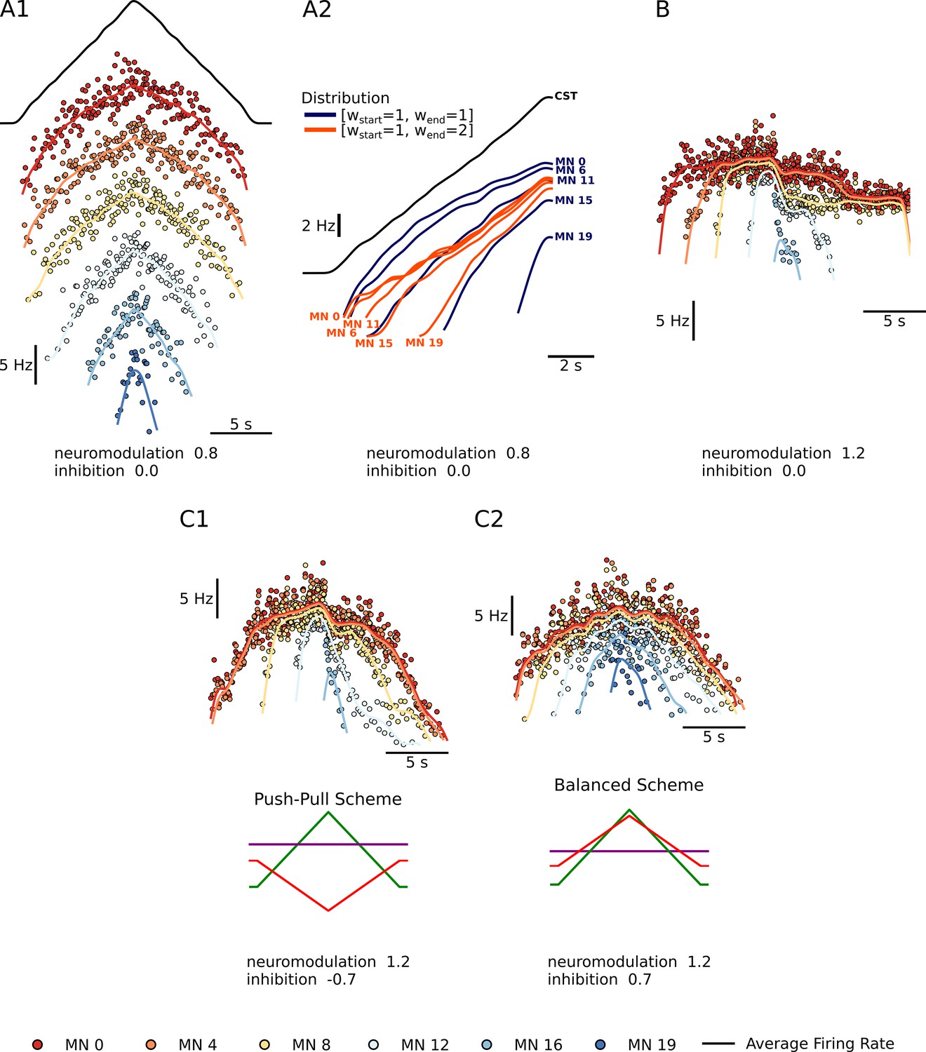
Summary plots showing the performance of the motoneuron pool model with respect to the integration of inputs.
(A1) - Shows a subset of 6 of the 20 motoneuron (MN) in the pool given the same excitatory triangular input, the black trace above. The MN pool follows an orderly activation known as the Henneman’s size principle, showing that this MN model can transform a ‘common drive‘ into different MN activities (see section Common input structure, differences in motoneuron properties). (A2) - Shows the model’s ability to favor S-type vs F-type motoneuron within the pool. The orange Distribution favors the fast (F-type) motoneuron. The recruitment of theses F-type motoneurons (e.g. MN 11, MN 15, and MN 19) happens sooner and their maximum firing rates are higher with respect to their counterparts. For the slow (S-type) motoneurons the recruitment is the same but their max firing rates decrease with respect to their counterparts (see section Distribution of excitatory input to S vs F motoneurons). (B) - Shows our model’s ability to trigger PIC-type behavior. For a neuromodulation level of 1.2 (max of range tested) and no inhibition, the motoneurons firing rates show a fast rise time, then attenuation, followed by sustained firing (see section Neuromodulation and excitatory input). (C1 and C2) - Shows the model’s ability to modulate the effects of neuromodulation with inhibition. (C1) shows an inhibition in the ‘Push-Pull’ or reciprocal configuration. (C2) shows inhibition in the balanced configurations (see section Neuromodulation and inhibition).
Figure 2
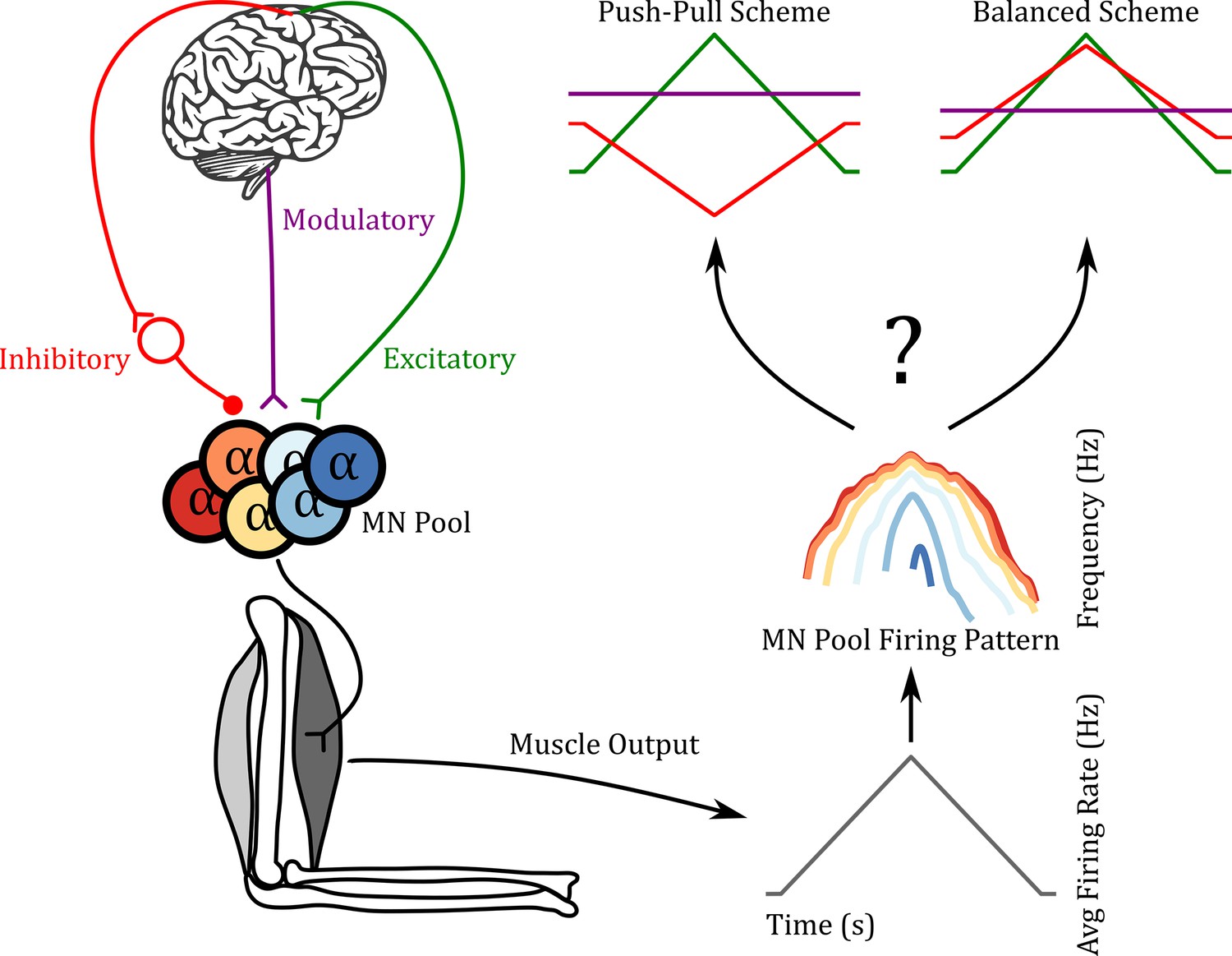
Reverse engineering paradigm.
The left side shows a schematic of the input pathway to the motoneuron (MN) pool and its subsequent connection to a muscle. The right side shows a schematic of our goal. Can we predict the three inputs of the MN pool given the firing pattern of the MN pool used to generate the muscle output? In the push-pull scheme at the upper right, inhibition (red) decreases as excitation (green) increases. In contrast, inhibition increases with excitation in the balanced scheme. In this work, we show that using the ‘MN Pool Firing Pattern’ one is able to reverse engineer back to the MN pool inputs.
Figure 3
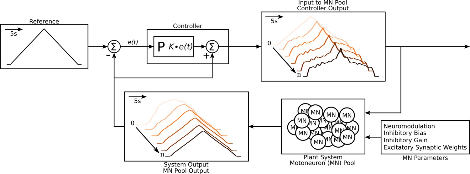
Schematic of the algorithm used to approximate the excitatory input needed to produce the triangular output from the motoneuron pool.
The schematic resembles a classic controller schematic. The algorithm starts at the ‘Input to motoneuron (MN) Pool’ box where the light pink triangular input is used as the initial guess to the ‘Plant System‘ box. Using this initial input guess, the MN pool model calculates it first output, seen in the ‘System Output’ box (light pink trace). This initial output is compared to the ‘Reference’ Box and the resulting error is fed into the ‘Controller’ box. Based on this error the controller calculates a new guess for an input and the cycle is repeated until a satisfactory error is achieved (MSE <1 Hz2). The iterations are shown within the ‘Input to MN Pool‘ and ‘System Output’ boxes along a left-to-right diagonal scheme to show the evolution of the traces produced by the algorithm. From iteration 0 to iteration the input to the MN pool morphs to a highly non-linear form to produce a linear output. Finally, this algorithm is repeated over a range of neuromodulation, inhibitory bias, inhibitory gain, and excitatory synaptic weights as shown in the ‘MN parameters’ box. Taking all the iterations and combinations, the model was run at a total of 6,300,000 times. See subsection Simulation protocol for details.
Figure 4
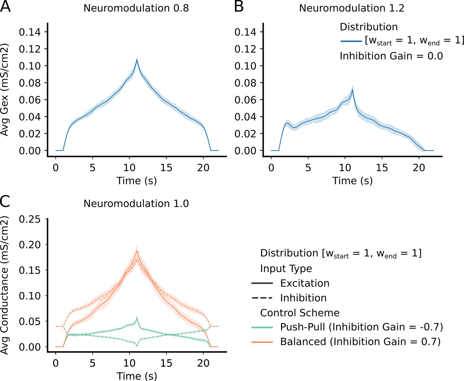
Top Row – shows the average and std excitatory input to the motoneuron (MN) pool to produce the reference command (Figure 3 – reference input).
(A) has a neuromodulation value of 0.8. (B) has a neuromodulation value of 1.2. For both (A) and (B), the inhibitory gain is set to zero and the excitatory weight distribution is equal across the pool (111 configuration - see section Excitatory distribution or MN weights). In short, the lower the neuromodulation the more linear the input command becomes however, the higher the excitatory values becomes. Bottom Row - (C) - shows the average and std excitation (solid) and inhibition (dotted) for the two extremes of inhibitory schemes (Push-pull in green and Balanced in orange). Neuromodulation is set to 1.0 (middle of range tried) and the excitatory weight distribution is equal across the pool (111 configuration - see section Excitatory distribution or MN weights). The "Push-Pull" inhibitory scheme requires less overall drive to achieve the same output.
Figure 5
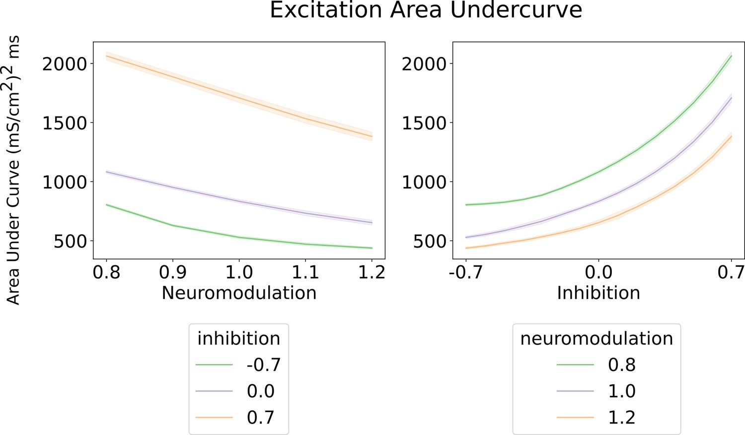
Area under the curve for the excitatory inputs calculated by the algorithm (Figure 3 and Methods).
Left - Shows the area under the curve of the excitatory input with respect to neuromodulation and inhibitory levels (color scheme). Their inhibitory levels are clearly segregated across the neuromodulation range. The most efficient inhibitory scheme is ‘Push-pull‘ (–0.7) and the least is ‘Balanced’ (0.7). Right - shows the area under the curve of the excitatory input with respect to inhibition for three neuromodulation level. The curves for each neuromodulation level do not intersect across the range of inhibition. The overall trend resembles the results on the left where the most efficent scheme is for high neuromodulation (1.2) and a ‘Push-pull’ inhibition (–0.7). These curves were calculated using an equally weighted excitatory input.
Figure 6
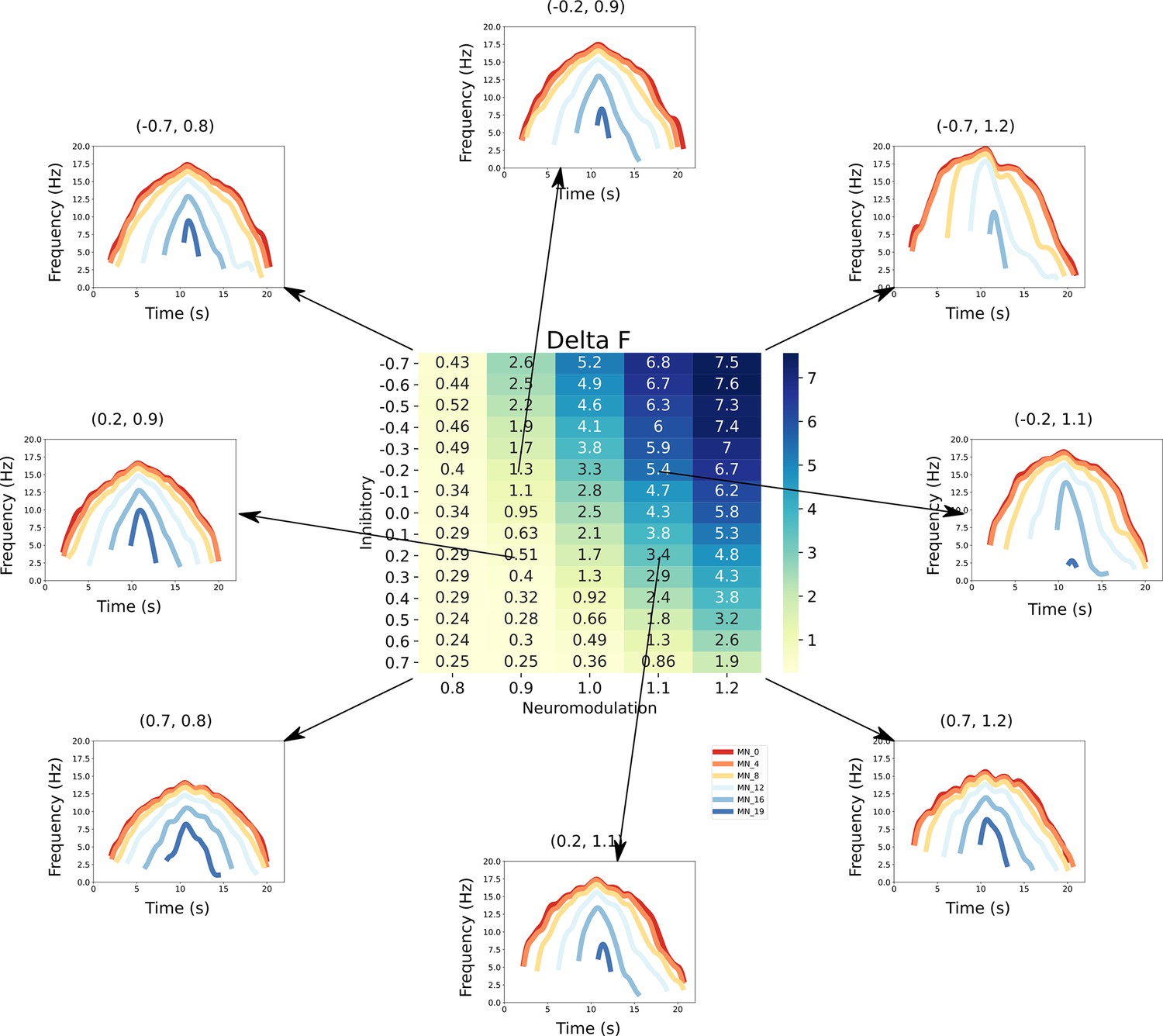
This figure links the firing rate shapes of the motoneuron (MN) pool model to the inhibitory and neuromodulatory search space.
Heat Map - The central figure is a heat map of the mean values of the MN pool model calculated using the firing rate patterns of the motoneurons in the MN pool model (see section Feature extraction). These values are organized along the neuromodulation (x-axis) and inhibitory values (y-axis) used in the simulations. Firing Rate Plots - Emanating from the central figure are a subset of the firing rate plots of the MN pool model given a specific Inhibitory and Neuromodulation set (e.g. (0.2, 0.9)). These plots are linked to a value with an arrow. For clarity, only a subset of motoneuron firing rates are shown. From visual inspection, the shape of the firing rates differ given the Inhibition and Neuromodulation pair, from more non-linear (e.g. (–0.7, 1.2)) to more linear (e.g. (0.2, 0.9)).
Figure 7

Features extracted from the firing rate patterns of each of the motoneurons in the pool.
We extracted the following seven features: Recruitment Time (), De-Recruitment Time (), Activation Duration (), Recruitment Range (), Firing Rate Saturation (), Firing Rate Hysteresis (), and brace–height (brace–height). These features are then used to estimate the neuromodulation, inhibition, and excitatory weights of the motor pool (see section Machine learning inference of motor pool characteristics and Regression using motoneuron outputs to predict input organization). See the subsection Feature extraction for details on how to extract features.
Figure 8
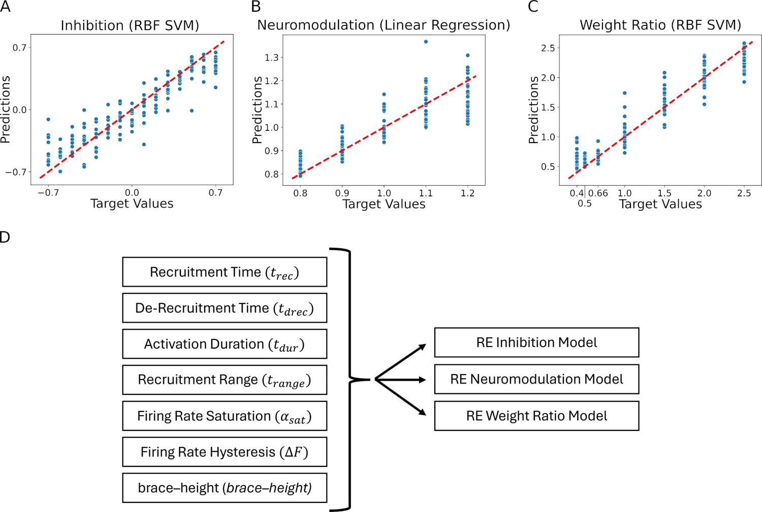
Residual plots showing the goodness of fit of the different predicted values: (A) Inhibition, (B) Neuromodulation, and (C) excitatory Weight Ratio.
The summary plots are for the models showing the highest results in Table 1. The predicted values are calculated using the features extracted from the firing rates (see Figure 7, section Machine learning inference of motor pool characteristics and Regression using motoneuron outputs to predict input organization). Diagram (D) shows the multidimensionality of the reverse engineering (RE) models (see Model fits) which have seven feature inputs (see Feature Extraction) predicting three outputs (Inhibition, Neuromodulation, and Weight Ratio).
Figure 9
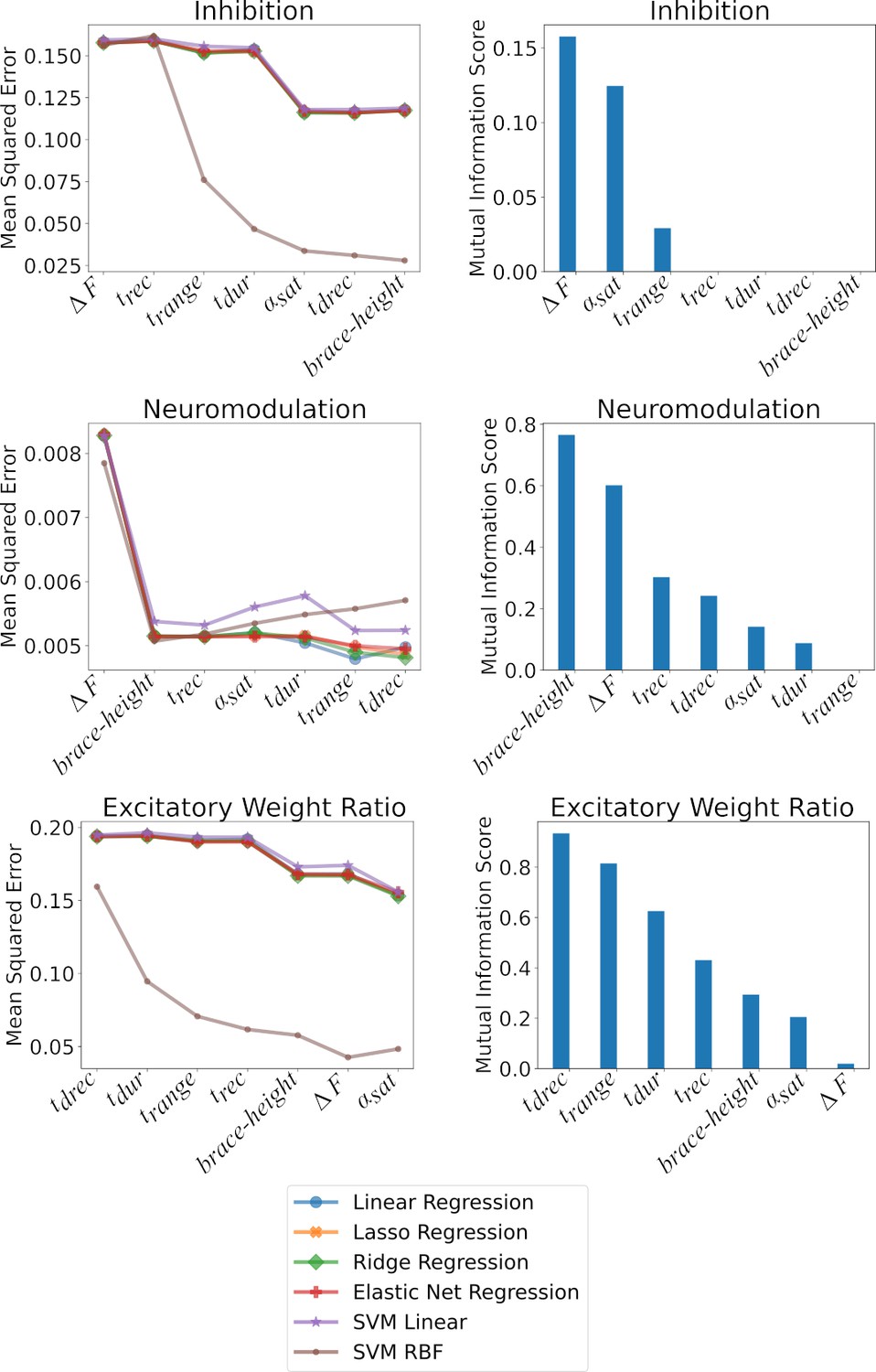
Shows the impact of the features on the models at predicting Inhibition, Neuromodulation, and the excitatory Weight Ratios.
The plots are split along two columns showing two types of complementary analysis: F-Statistic (left) and Mutual Information (right). Left - The left column shows the impact of the features on the MSE as ranked by their value. The effect of the features are cumulative along the x-axis such that the value of the MSE at a given position in the x-axis is calculated using the features up to that point. Each of the colored traces represents one of the models used to predict the three outcomes and follows the trends found in Table 1. Right - The right column shows the mutual information of each feature with respect to the outcome: Inhibition, Neuromodulation, and excitatory Weight Ratio (Top to Bottom). The features are ranked from best to worst along the x-axis. The ranking matches the MSE ranking in the right column. See the section Ranking features to see details on how these techniques were implemented.
Appendix 2—figure 1
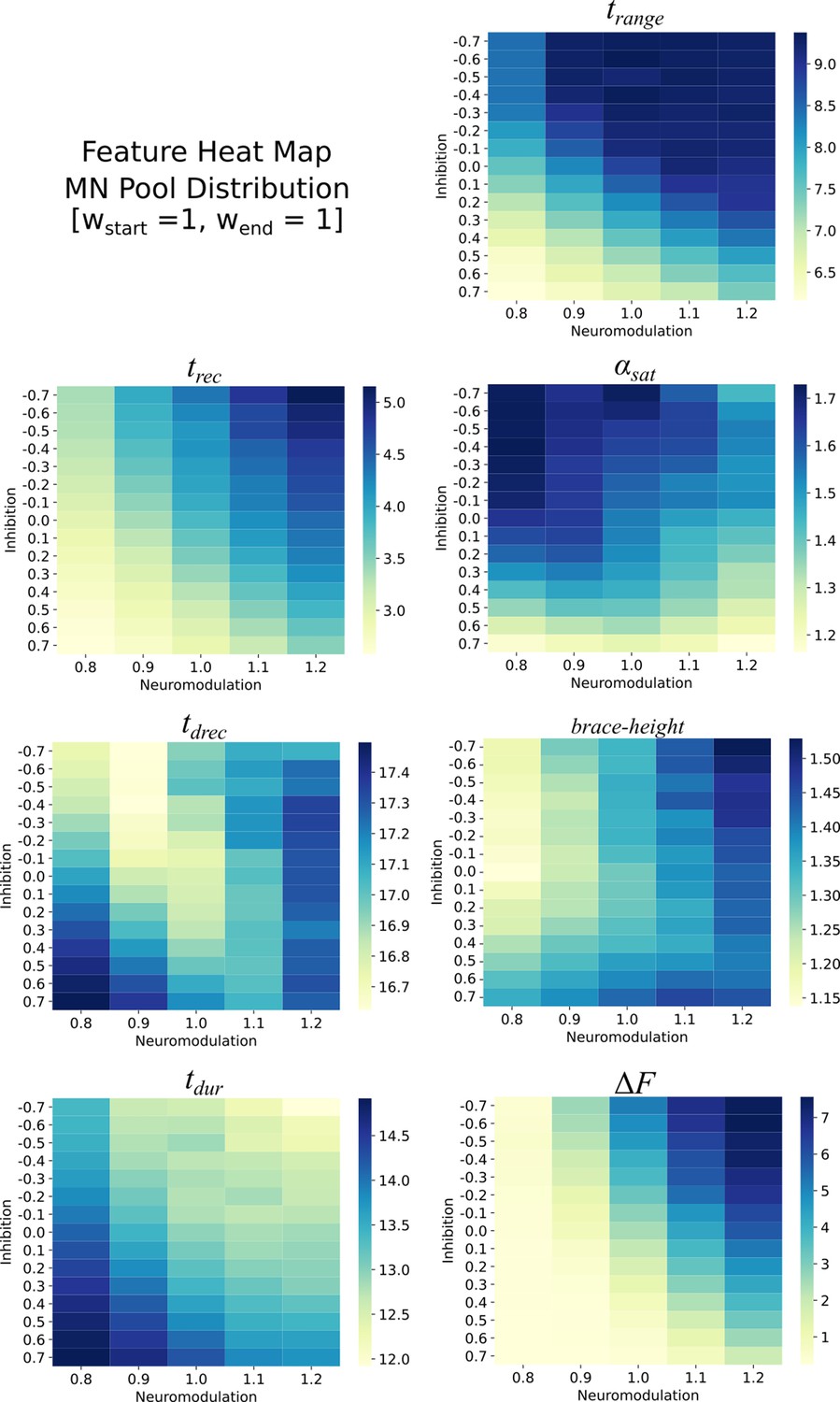
Heat maps for the different features extracted from the firing rates of the monotoneurons in the pool model.
These heat maps are for the equally distributed excitatory weights . Each heat map is organized along the Neuromodulation and Inhibitory ranges tried in this work. The values within these heat maps show structure with respect to Neuromodulation and Inhibition and show that this structure can be used to reverse engineer the Neuromodulation and Inhibition themselves.
Appendix 2—figure 2

Schematic of the parallel architecture used to solve the motoneuron (MN) pool model and to find the solution for the input to that pool.
Each neuromodulation, inhibition, excitatory input weight, and noise seed combination was assigned a node on the computer via the slurm batch scheduler. These ‘hyper-parameters’ were passed to each motoneuron which had a dedicated CPU core using the message passing interface (MPI). This work was done on the Bebop supercomputer at Argonne National Laboratory, Lemont, IL.
Author response image 1

Figure 8.
Residual plots showing the goodness of fit of the different predicted values: (A) Inhibition, (B) Neuromodulation and (C) excitatory Weight Rao. The summary plots are for the models showing highest 𝑅𝑅2 results in Table 1. The predicted values are calculated using the features extracted from the firing rates (see Figure 7, section Machine learning inference of motor pool characteristics and Regression using motoneuron outputs to predict input organization). Diagram (D) shows the multidimensionality of the RE models (see Model fits) which have 7 feature inputs (see Feature Extraction) predicting 3 outputs (Inhibition, Neuromodulation and Weight Rao).
Tables
Table 1
values.
Rows are the predicted values. Columns are the models. The values in bold represent the best model fit: Inhibition is best predicted using the radial basis function kernel (RBF) SVM model, Neuromodulation is best predicted by the Ridge model, and Excitation Weight Ratio is best predicted by the RBF SVM model.
| Name | Linear regression | Lasso | Ridge | Elastic net | Linear SVM | RBF SVM |
|---|---|---|---|---|---|---|
| Inhibition | 0.36 | 0.36 | 0.36 | 0.36 | 0.35 | 0.85 |
| Neuromodulation | 0.75 | 0.76 | 0.76 | 0.75 | 0.74 | 0.71 |
| Excitation Weight Ratio | 0.72 | 0.72 | 0.72 | 0.72 | 0.72 | 0.91 |
| Average | 0.61 | 0.61 | 0.61 | 0.61 | 0.60 | 0.83 |
Additional files
Download links
A two-part list of links to download the article, or parts of the article, in various formats.
Downloads (link to download the article as PDF)
Open citations (links to open the citations from this article in various online reference manager services)
Cite this article (links to download the citations from this article in formats compatible with various reference manager tools)
Supercomputer framework for reverse engineering firing patterns of neuron populations to identify their synaptic inputs
eLife 12:RP90624.
https://doi.org/10.7554/eLife.90624.3


