Microphase separation produces interfacial environment within diblock biomolecular condensates
Figures
Figure 1
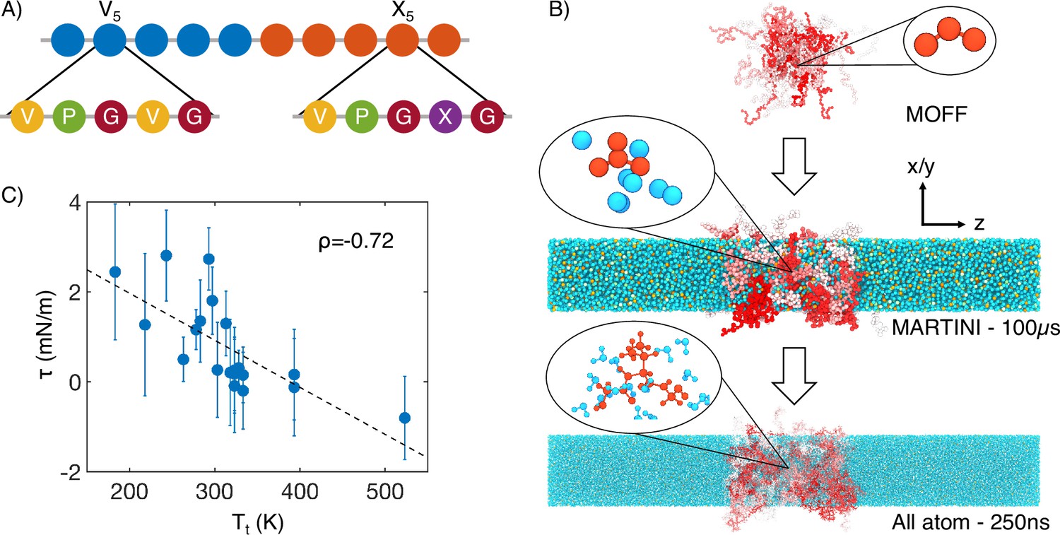
Multiscale simulations enable thermodynamic and structural characterization of elastin-like polypeptide (ELP) condensates.
(A) Illustration of the sequence for the simulated diblock ELPs that consist of five-amino acid repeats, where X is substituted with a guest amino acid. (B) Overview of the three-step multiscale simulation approach that gradually increases the model resolution. Simulations of V5L5 were used to produce the example configurations at each step. Peptides are shaded red-white, while water molecules, chlorine, and sodium are colored in blue, green, and orange, respectively. Inserts of a G-V-G repeat and surrounding water molecules are shown to indicate the resolution of each model. (C) Correlation between the simulated surface tension () of 20 ELP condensates and the transition temperatures () of related systems (Urry, 1997) is the Pearson correlation coefficient between the two data sets, and the dashed line is the best fit between simulation and experimental data. Error bars represent the SD of estimates from five independent time windows.
Figure 2 with 7 supplements
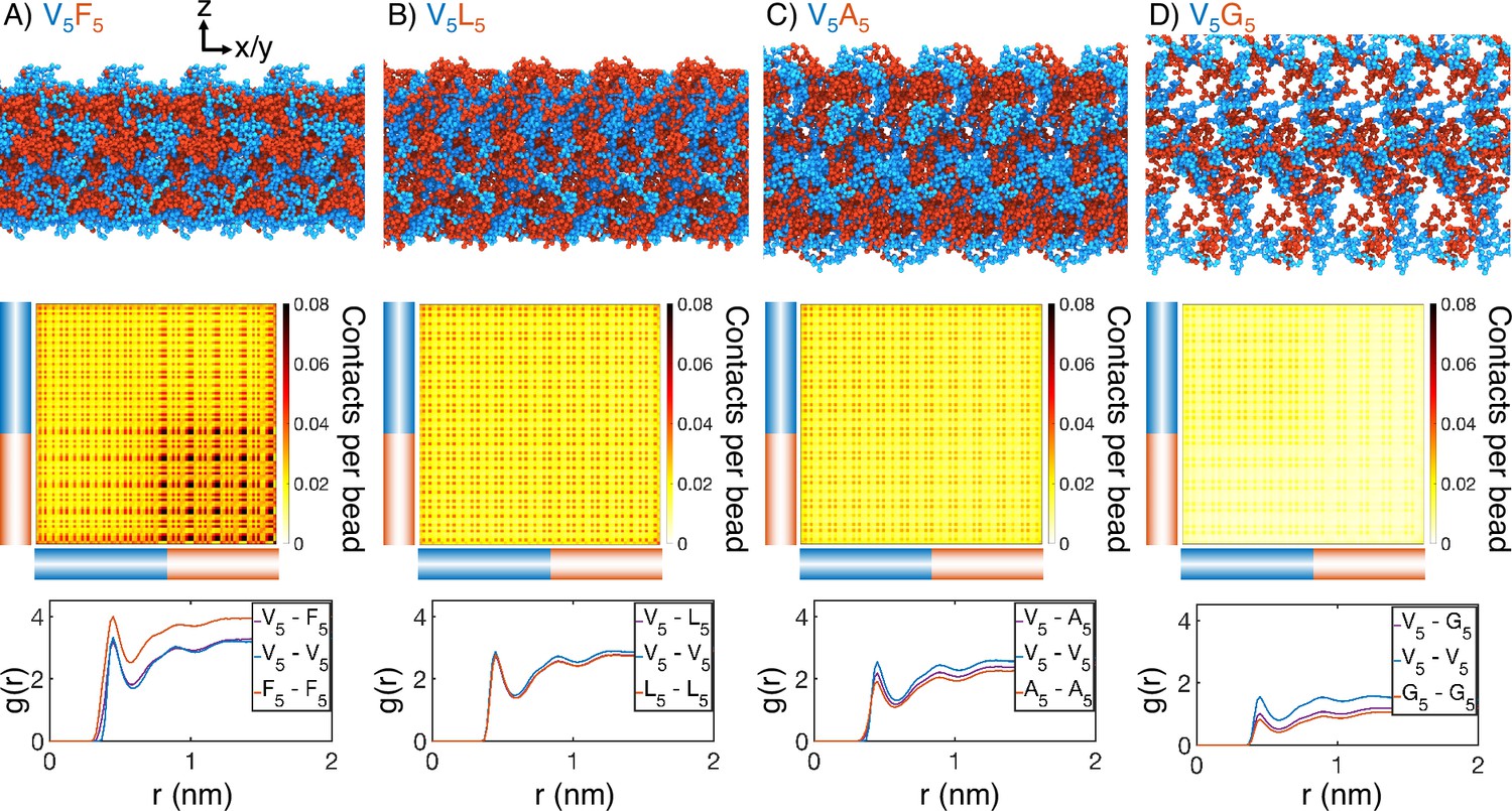
Internal organization of elastin-like polypeptide (ELP) condensates for (A) V5F5, (B) V5L5, (C) V5A5, and (D) V5G5.
The uppermost panels present representative configurations from MARTINI simulations for each system. Periodic images along the x and y dimensions are shown for clarity, and the condensate-water interface is perpendicular to the z-axis. Only proteins are shown, with the X- and V-substituted halves of the peptides shown in red and blue, respectively. The central panels show contact maps between amino acids from different peptides. The blue and red bars indicate the V- and X-substituted half of the peptides. The lower panels plot the radial distribution functions, , for amino acids only from the V-substituted half of the peptides (V5-V5), only from the X-substituted half of the peptides (X5-X5), and between the two halves (V5-X5). We limited the calculations to amino acid pairs from different peptides.
Figure 2—figure supplement 1
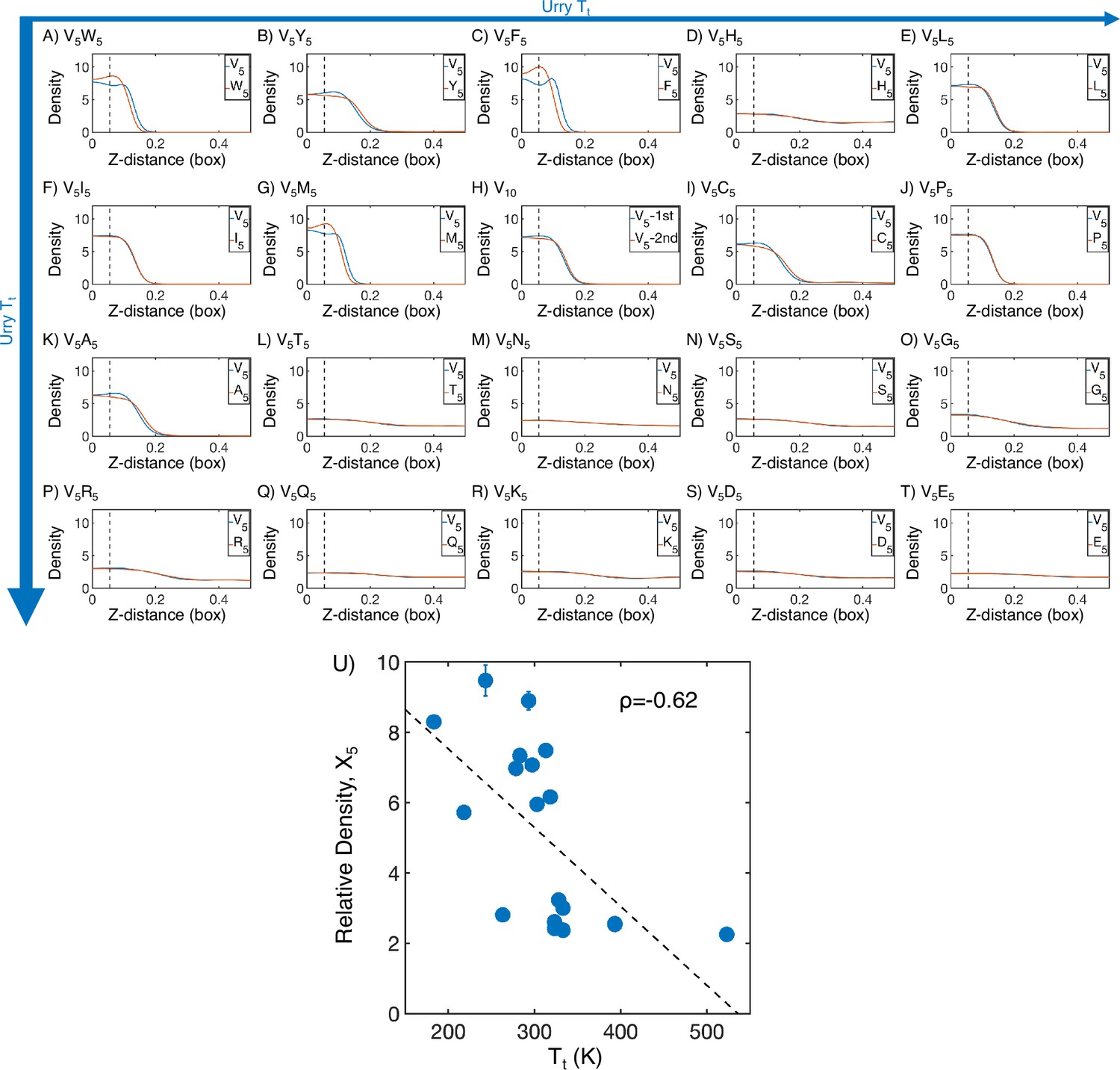
Mass density profiles of elastin-like polypeptide (ELP) condensates from MARTINI simulations.
(A–T) The relative mass density along the Z-distance from the condensate center is shown for the V-substituted and X-substituted halves of each condensate. The Z-axis is defined as the direction perpendicular to the condensate-water interface. The dashed line represents a Z-distance of 0.06 box lengths away from the condensate center. Average density values below this threshold are used for correlation analysis in (U). Proteins are arranged by increasing (decreasing hydrophobicity) from Urry, 1997 with (A, V5W5) being the most hydrophobic and (T, V5E5) being the least hydrophobic. (U) Correlation between the mass fraction of the X5 half of the condensate and transition temperature () from Urry, 1997. is the Pearson correlation coefficient between the two data sets, and the dashed diagonal line is the best-fit line. Error bars represent SDs of the mean taken over six equally spaced box length intervals.
Figure 2—figure supplement 2
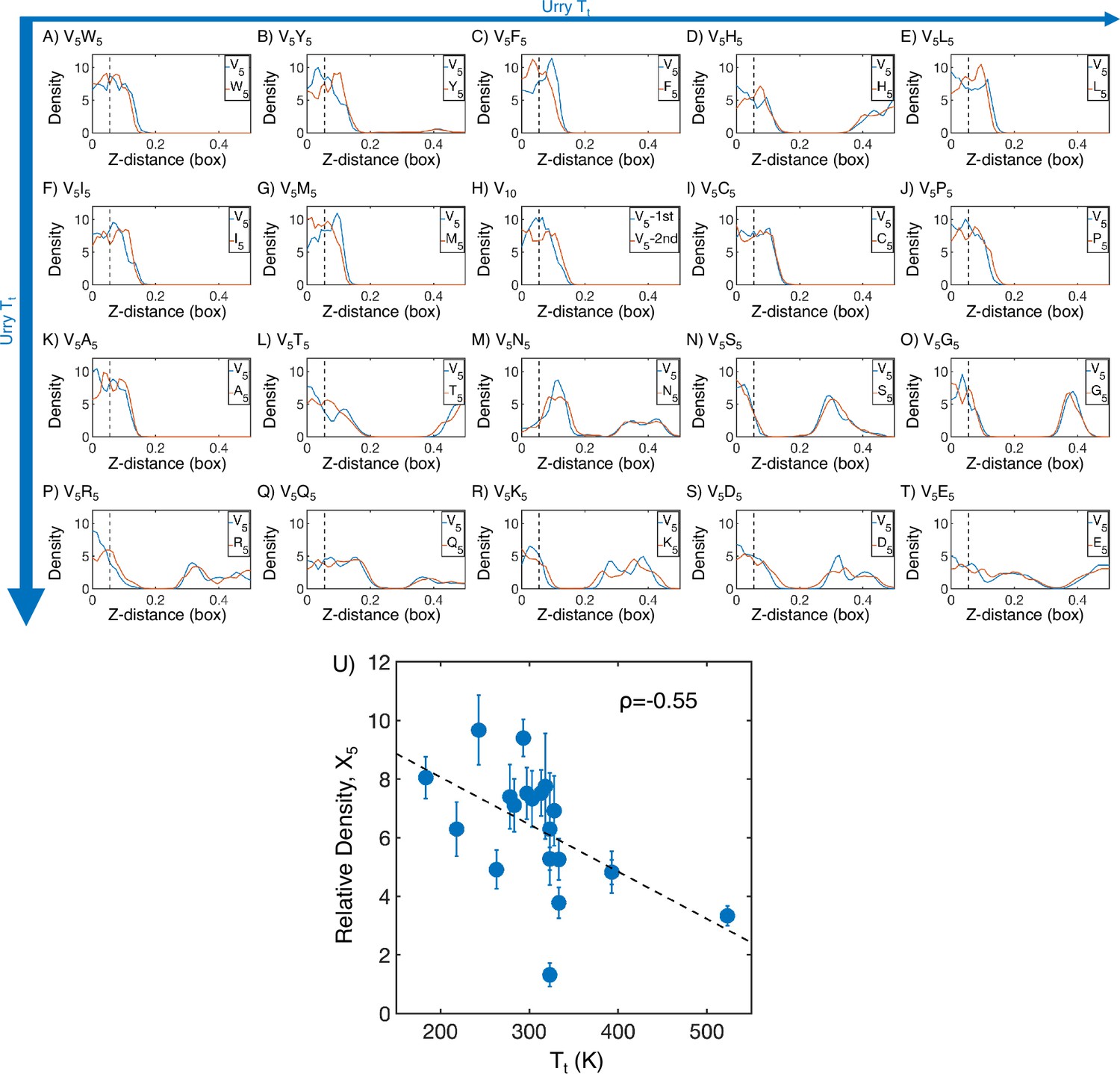
Mass density profiles of elastin-like polypeptide (ELP) condensates from all-atom simulations.
(A–T) The relative mass density along the Z-distance from the condensate center is shown for the V-substituted and X-substituted halves of each condensate. The Z-axis is defined as the direction perpendicular to the condensate-water interface. The dashed line represents a Z-distance of 0.06 box lengths away from the condensate center. Average density values below this threshold are used for correlation analysis in (U). Proteins are arranged by increasing (decreasing hydrophobicity) from , Urry, 1997 with (A, V5W5) being the most hydrophobic and (T, V5E5) being the least hydrophobic. (U) Correlation between the mass fraction of the X5 half of the condensate and transition temperature () from Urry, 1997. is the Pearson correlation coefficient between the two data sets, and the dashed diagonal line is the best-fit line. Error bars represent SDs of the mean taken over six equally spaced box length intervals.
Figure 2—figure supplement 3
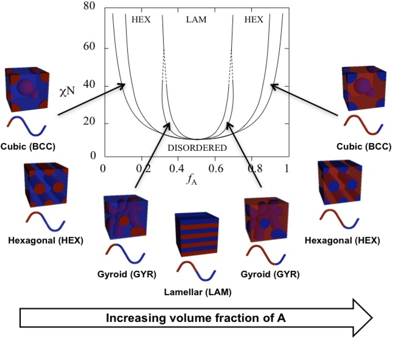
Theoretical phase diagram (Matsen and Bates, 1996) and corresponding morphologies for diblock copolymers.
The phases are labeled as body centered cubic (BCC), hexagonal cylinders (HEX), gyroid (GYR), and lamellar (LAM). is the volume fraction of a single polymer block, denoted A, is the Flory–Huggins interaction parameter, and is the total degree of polymerization. Reproduced from Figure 3 from Swann and Topham, 2010 (CC BY 4.0).
Figure 2—figure supplement 4
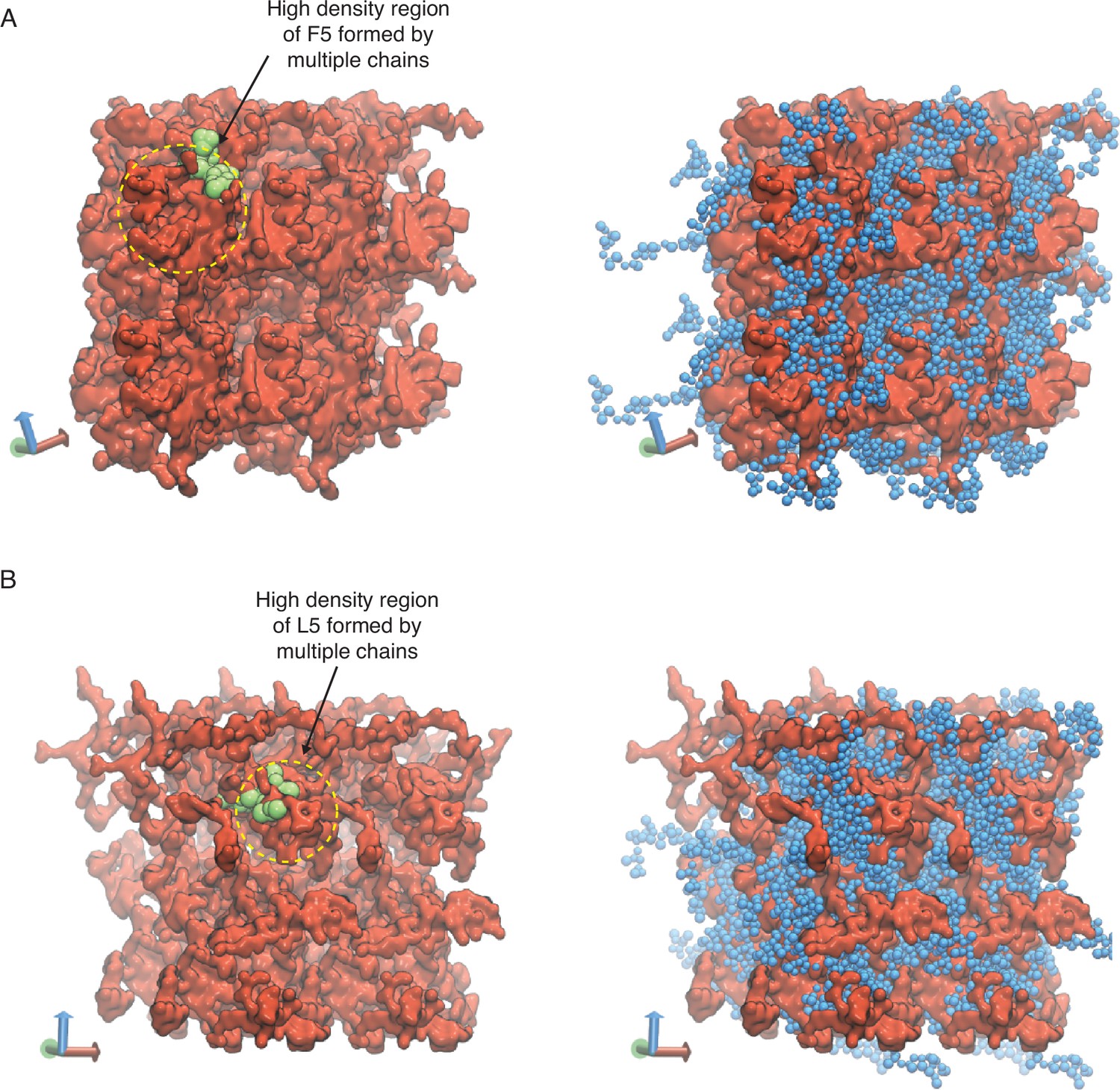
Representative configurations of (A) V5F5 and (B) V5L5 condensates from MARTINI simulations.
The valine substituted half of the chain is colored blue (V5) and the X-substituted half of the chain is colored red (X5). To highlight the interpenetrating networks formed by the two halves, only the X-substituted half of the chain is shown on the left. Simulation interfaces are once repeated periodically in the positive x and positive y dimensions for clarity. High-density regions formed by the multiple X-substituted half of the chains are highlighted in yellow circles, with one of the chain shown in green.
Figure 2—figure supplement 5
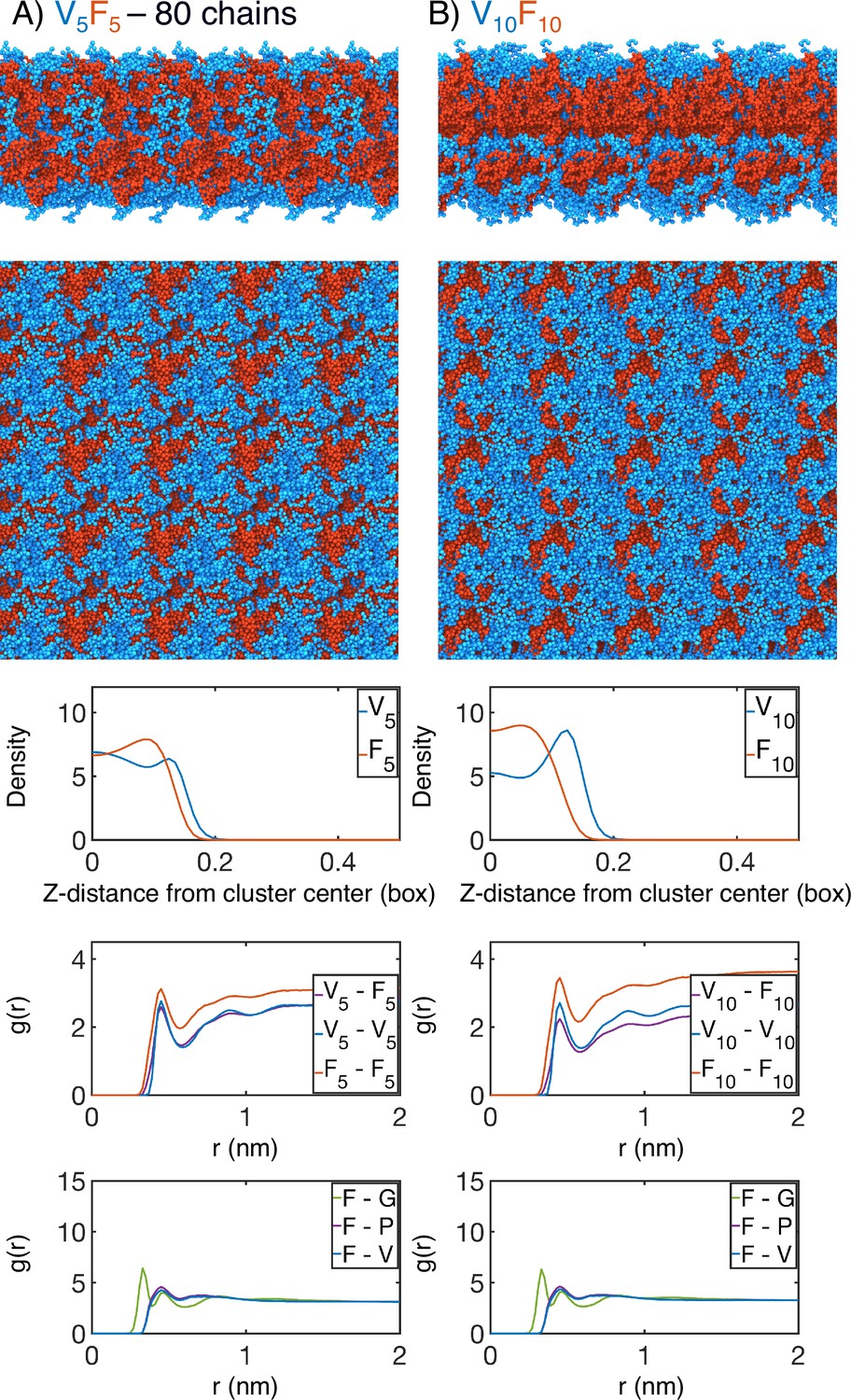
Finite size effect checks of our simulation methodology by (A) doubling the number of chains in the simulation box (V5F5 ; 80 chains) or by (B) doubling the length of the peptide sequence (V10F10).
In each case, the uppermost panel is a periodic image of the simulated condensate. Only the protein is shown, with red highlighting the X-substituted half of the condensate and blue highlighting the V-substituted half of the condensate. The second panel from the top is condensate viewed from the simulation interface. The middle panel is the mass density from the condensate center for the V-substituted and X-substituted halves of each condensate. The second panel from the bottom is the radial distribution function g(r) for inter-chain coarse-grained beads, divided between the V5 half of the chain and X5 half of the chain. The bottom panel is the overall radial distribution function from the guest amino acid (X5), to those amino acids native to the ELP sequence.
Figure 2—figure supplement 6
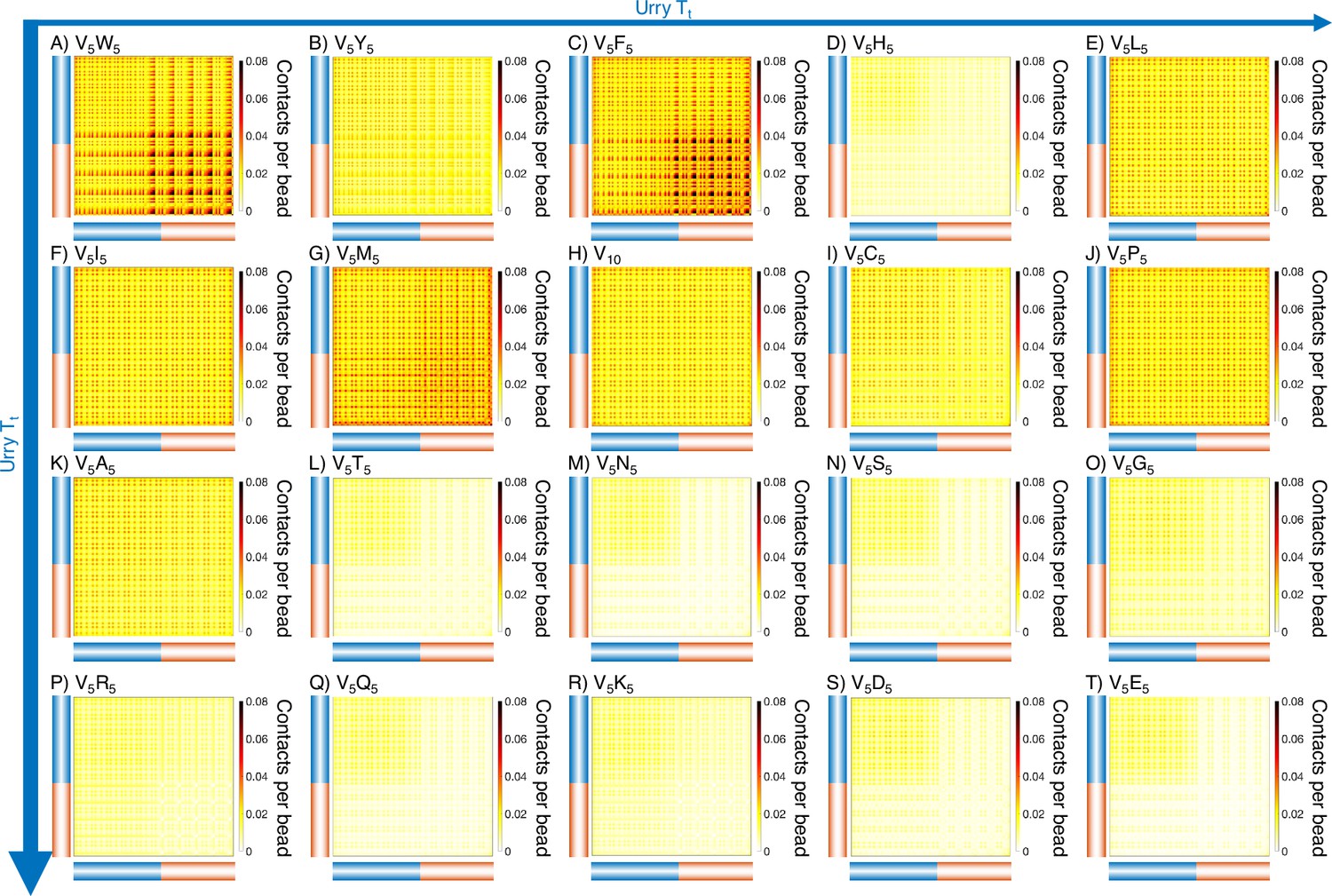
Intermolecular contact maps for elastin-like polypeptide (ELP) peptides from MARTINI simulations.
The blue bar highlights the V5 half of the condensate, while red bar highlights the X5 half. Proteins (A-T) are arranged by increasing (decreasing hydrophobicity) from Urry, 1997 with (A, V5W5) being the most hydrophobic and (T, V5E5) being the least hydrophobic.
Figure 2—figure supplement 7
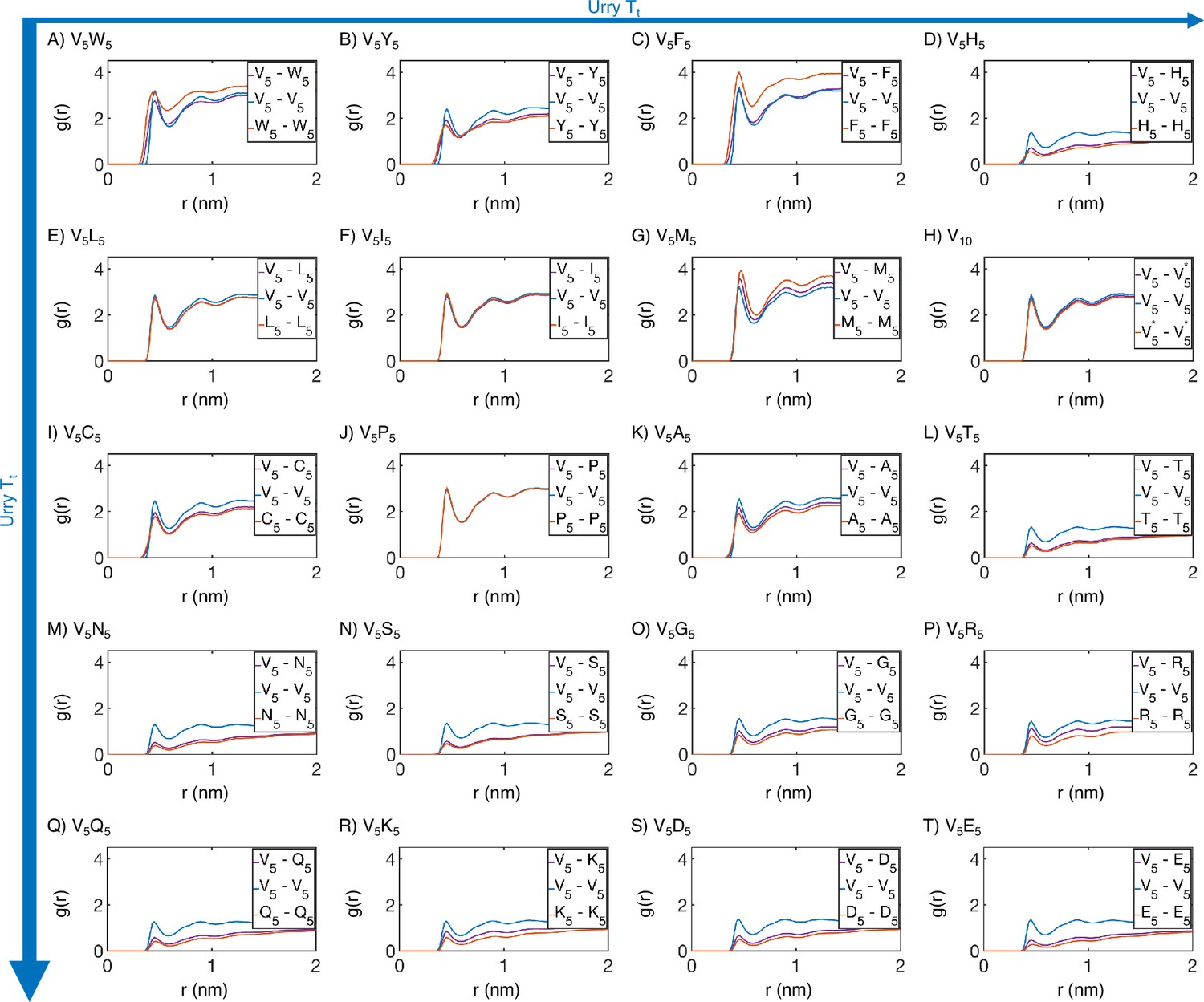
Radial distribution functions from MARTINI simulations support the microphase separation of different elastin-like polypeptide (ELP) blocks.
Amino acids from the V5 and X5 half of the ELP peptide are partitioned into two blocks, and we used distances within and across the blocks to compute . Distances between amino acids from the same peptide are excluded from computations. Proteins (A-T) are arranged by increasing (decreasing hydrophobicity) from Urry, 1997, with (A, V5W5) being the most hydrophobic and (T, V5E5) being the least hydrophobic.
Figure 3 with 2 supplements
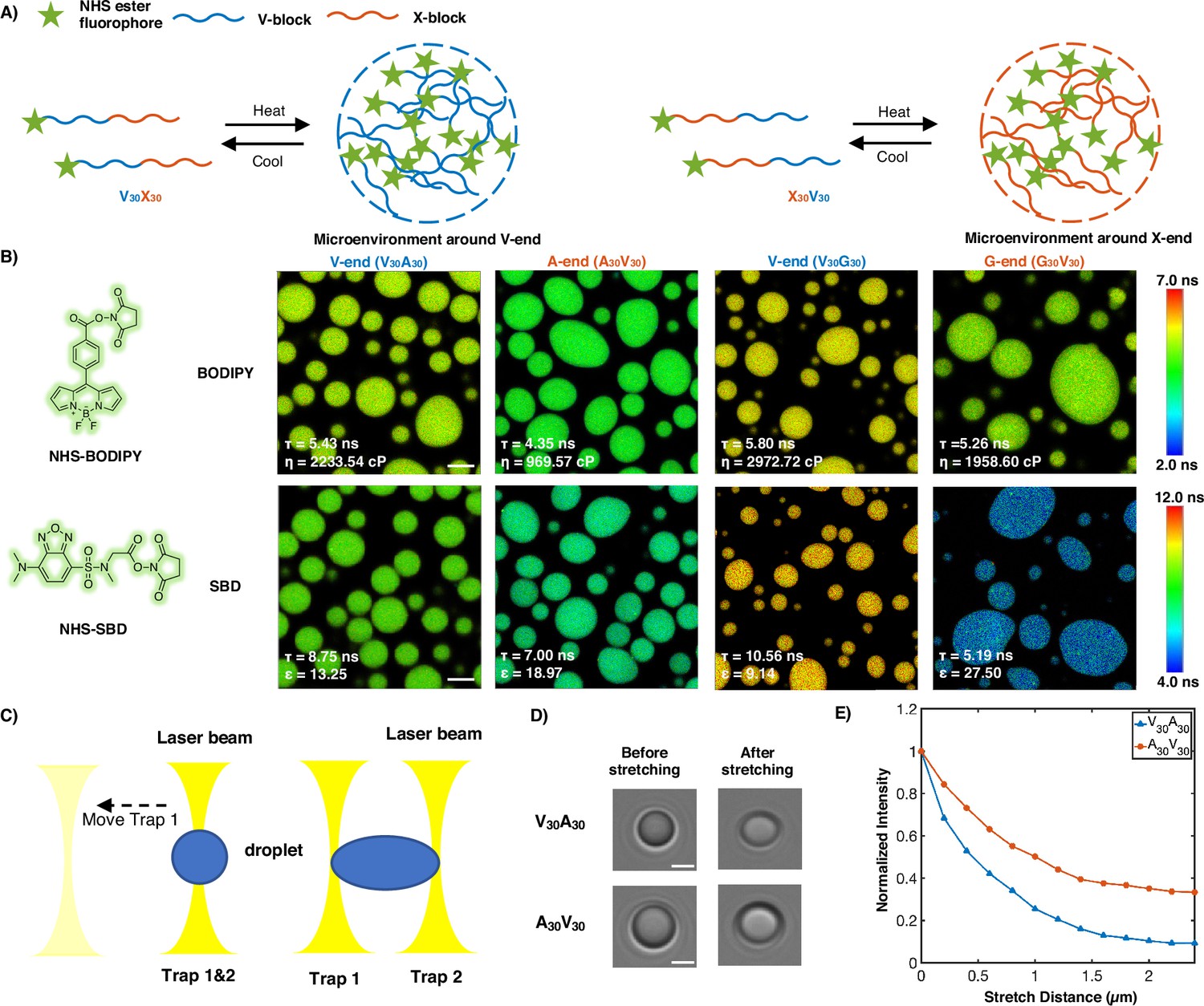
Experimental support of the microphase separation of elastin-like polypeptide (ELP) condensates.
(A) Reversible ELP condensates formation via changing temperature. NHS ester fluorophores are attached at the amino-termini of V30X30 and X30V30 to detect the different micro-physicochemical properties between the V-end and the X-end. (B) Structures of NHS-BODIPY and NHS-SBD, and FLIM images of V30A30, A30V30, V30G30, and G30V30 labeled with respective fluorophores. The fluorescence lifetime of each image is the average acquired from three independent experiments. Scale bar: 5 μm. (C) Schematic diagram of optical tweezers stretching experiment. (D) Bright-field images of V30A30 and A30V30 in the stretching experiment using the optical tweezer. Scale bar: 2 μm. (E) Normalized droplets fluorescence intensity changes while stretching (red curve: V30A30; blue curve: A30V30). Fifteen droplets (at size ∼4 μm) were imaged and used for statistical analysis.
Figure 3—figure supplement 1
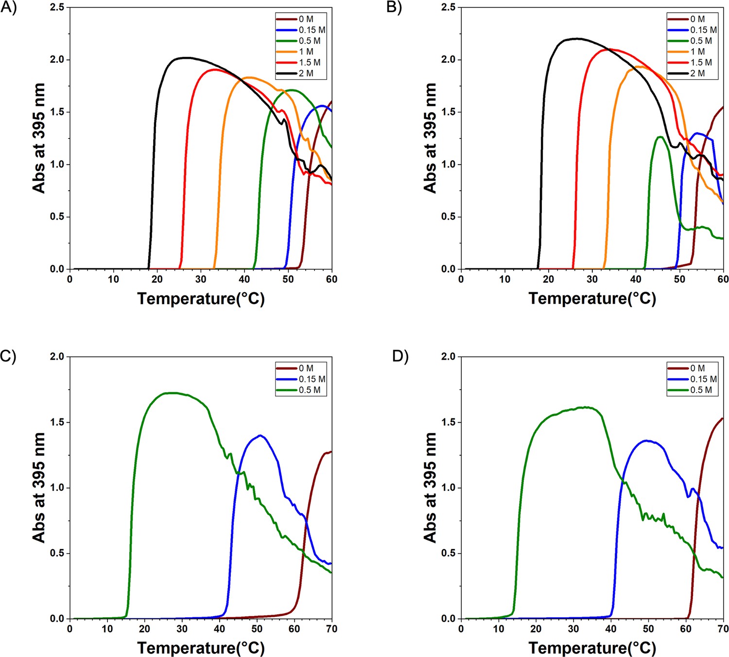
Experimental of elastin-like polypeptide (ELP) sequences.
The diagram of (A) V30A30, (B) A30V30, (C) V30G30, and (D) G30V30. The turbidity was measured in the NaCl solution with different concentrations for V30A30 and A30V30 and in (NH4)2SO4 solution with different concentrations for V30G30 and G30V30. The heat-up rate is 0.5°C/min, and absorbance data were collected every 0.5°C.
Figure 3—figure supplement 2
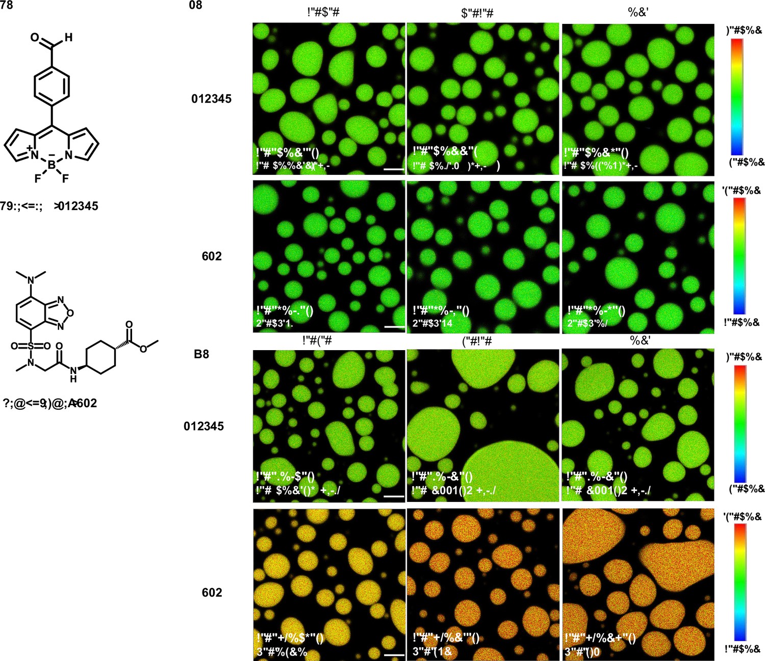
Fluorescence lifetime imaging microscopy (FLIM) image of unlabeled elastin-like polypeptide (ELP) condensates.
(A) Chemical structure of free fluorophore, which can measure the physicochemical properties of condensates without labeling. (B) Representative FLIM images of V30A30 and A30V30. The mix is the mixture of V30A30 (35 μM) and A30V30 (35 μM). Droplets were formed with a final concentration of 70 μM ELP in 2 M NaCl solution with 1 μM fluorophore. (C) Representative FLIM images of V30G30 and G30V30. Droplets were formed with a final concentration of 70 μM ELP in 1.5 M (NH4)2SO4 solution with 1 μM fluorophore. The mix is the mixture of V30G30 (35 μM) and G30V30 (35 μM). Scale bar, 5 μm. The fluorescence lifetime of each image is the average from three independent measurements.
Figure 4 with 1 supplement
Interior of elastin-like polypeptide (ELP) condensates exhibits interfacial properties as a result of microphase separation.
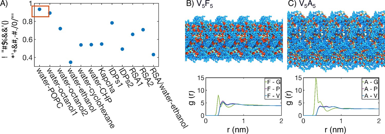
(A) Pearson correlation coefficient, , between the stated measure of hydrophobicity and the condensate transition temperature, , measured by Urry, 1997. To remove discrepancies in which end of the scale is hydrophobic and which end is hydrophilic, all hydrophobicity scales, including the Urry scale, are first normalized such that 1 corresponds to the most hydrophobic residue and 0 corresponds to the least hydrophobic residue. Hydrophobicity measures considered include experimental measures of water-solvent transfer free energies water-1-palmitoyl-2-oleoyl-sn-glycero-3-phosphocholine [POPC]-interface (White, 1996), water-octanol1 (Wimley et al., 1996), water-octanol2 (Wilce et al., 1995), water-ethanol (Zimmerman et al., 1968; Wilce et al., 1995), water-cyclohexane (Radzicka and Wolfenden, 1988), and water-N-cyclohexyl-2-pyrrolidone [CHP] (Lawson et al., 1984), atomic level analysis of moieties within amino acids (Kapcha and Rossky, 2014), computational approaches to estimate hydrophobicity within disordered proteins (IDPs1 Tesei et al., 2021 and IDPs2 Dannenhoffer-Lafage and Best, 2021), bioinformatics techniques that approximate the burial propensity, or relative solvent accessibility (RSA) of amino acids (RSA1 Rose et al., 1985 and RSA2 Tien et al., 2013), and a method that mixed protein burial fraction with water-vapor transfer free energy (RSA/water-vapor Kyte and Doolittle, 1982). The red box highlights the high correlation between and water-octanol or water-POPC interface transfer free energies. (B, C) Condensate organization from MARTINI simulations for V5F5 (B) and V5A5 (C). The top panels provide protein-only views for simulated condensates, with the guest residue X, glycine adjacent to the guest residue, and the remaining residues colored red, green, and blue, respectively. Condensate images are repeated periodically in the x/y plane. The bottom panel shows the overall radial distribution function from the guest amino acid to those amino acids native to the ELP sequence.
Figure 4—figure supplement 1
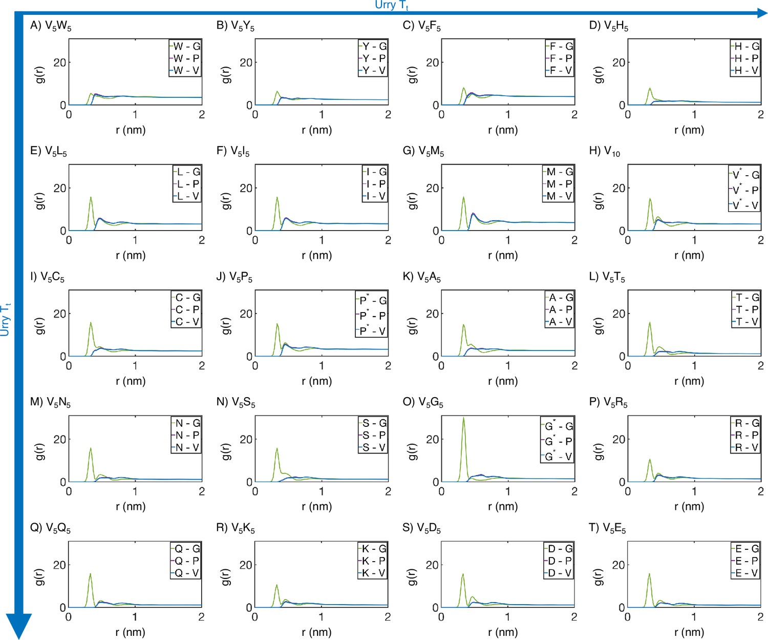
Residue-specific radial distribution function from MARTINI simulations.
Distances from the guest amino acid (X) to those amino acids native to the elastin-like polypeptide (ELP) sequence were used to compute . Substituted amino acids that also appear in the native sequence are differentiated from their native counterparts using a star (*). Proteins (A-T) are arranged by increasing (decreasing hydrophobicity) from Urry, 1997, with (A, V5W5) being the most hydrophobic and (T, V5E5) being the least hydrophobic.
Figure 5 with 1 supplement
Water hydrogen bonding environment of condensates from all-atom simulations.
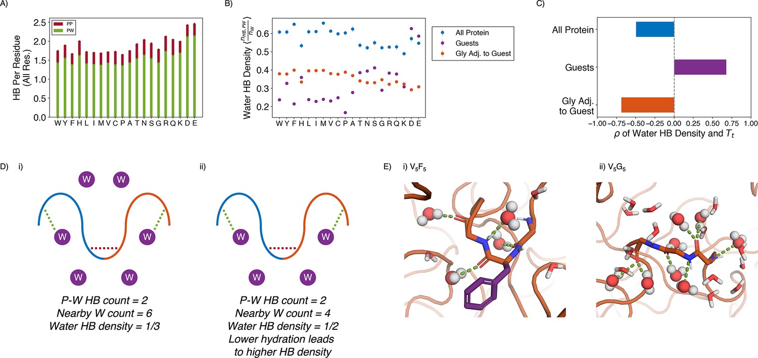
(A) Bar chart depicting the average number of protein-water (PW, in green) and protein-protein (PP, in red) hydrogen bond (HB) per residue for each condensate system. The x-axis presents the guest residue of the system and is ordered by the Urry scale. Error bars represent SDs of four independent estimates. (B) Water HB density for each of the 20 condensates, for three different residue selections. The metric is shown for all residues in the system (blue), guest residues (purple), and glycine residues adjacent to the guest residue in the sequence (orange). The x-axis presents the guest residue of the system and is ordered by the Urry scale. Error bars represent SDs of four independent estimates. (C) Correlation coefficients of the water HB density shown in (B) with Urry . (D) Schematics depicting two systems with low (i) and high (ii) water hydrogen bond density. The protein is depicted as blue and orange lines, and the water molecules are depicted as purple circles. Protein-protein and protein-water hydrogen bonds are drawn as red and green dashed lines respectively. (E) Visualizing hydrogen bond density with illustrative snapshots for V5F5 (i) and V5G5 (ii) condensate. Side chain carbon atoms are shown in purple. Water molecules near the protein are explicitly depicted, with oxygen and hydrogen atoms colored in red and white. Water molecules hydrogen bonded to the protein are depicted as spheres (with hydrogen bonds shown in green lines).
Figure 5—figure supplement 1
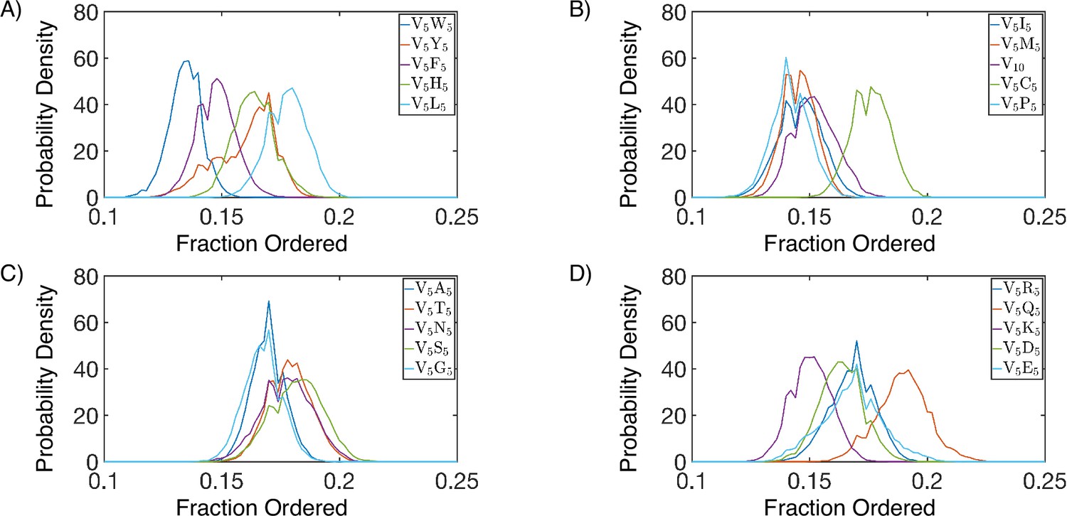
Secondary structure of simulated protein condensates, splitted into four panels (A-D), with protein names indicated in the legends.
Secondary structure is defined according to the DSSP algorithm (Touw et al., 2015; Kabsch and Sander, 1983). We consider α-helices, β-sheets, β-bridges, and turns as ordered, and display the total fraction of all these secondary structure elements for each simulated condensate.
Figure 6 with 1 supplement
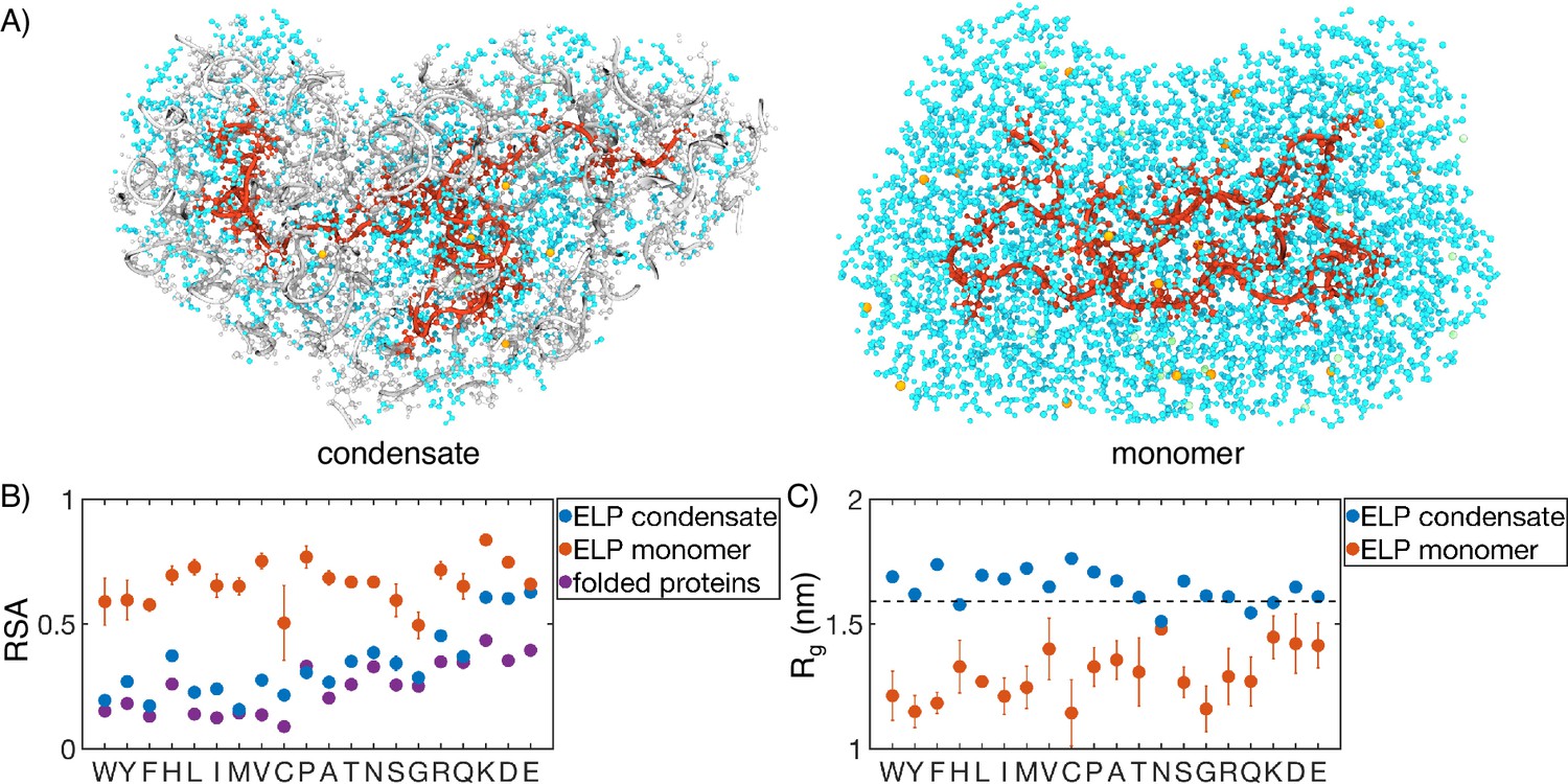
Comparison of protein conformation and solvation between elastin-like polypeptide (ELP) condensates and monomers.
(A) Zoom-in view of a single peptide chain (red) from atomistic simulations of V5A5 condensate (left) and monomer (right). Atoms within 1 nm of the peptide are shown, including water (cyan), chlorine (green), sodium (orange), and protein atoms from other chains (gray). (B) Relative solvent accessibility (RSA) of guest residues estimated from atomistic simulations of condensates (blue) and monomers (orange). For comparison, the corresponding values estimated using folded proteins are included as purple dots (Tien et al., 2013). Error bars represent the SD of four independent time estimates. (C) Comparison of the radius of gyration () for peptides estimated from atomistic simulations of condensates (blue) and monomers (orange). The dashed line represents the expected of an ideal chain, utilizing values that have been previously suggested for intrinsically disordered proteins (IDPs) (Hofmann et al., 2012; Dignon et al., 2018a). Error bars represent the SD of four independent time estimates.
Figure 6—figure supplement 1

of individual peptide blocks from MARTINI (A) and atomistic (B) simulations.
V5 represents the valine block, while X5 represents the guest block. Error bars represent SDs of the mean over four independent time windows. The dashed lines represent different values of polymer scaling exponents, with corresponding to an ideal chain and corresponding to a swollen polymer chain. Values previously suggested for intrinsically disordered proteins (IDPs) were used in calculation of the scaling exponent (Hofmann et al., 2012).
Appendix 1—figure 1
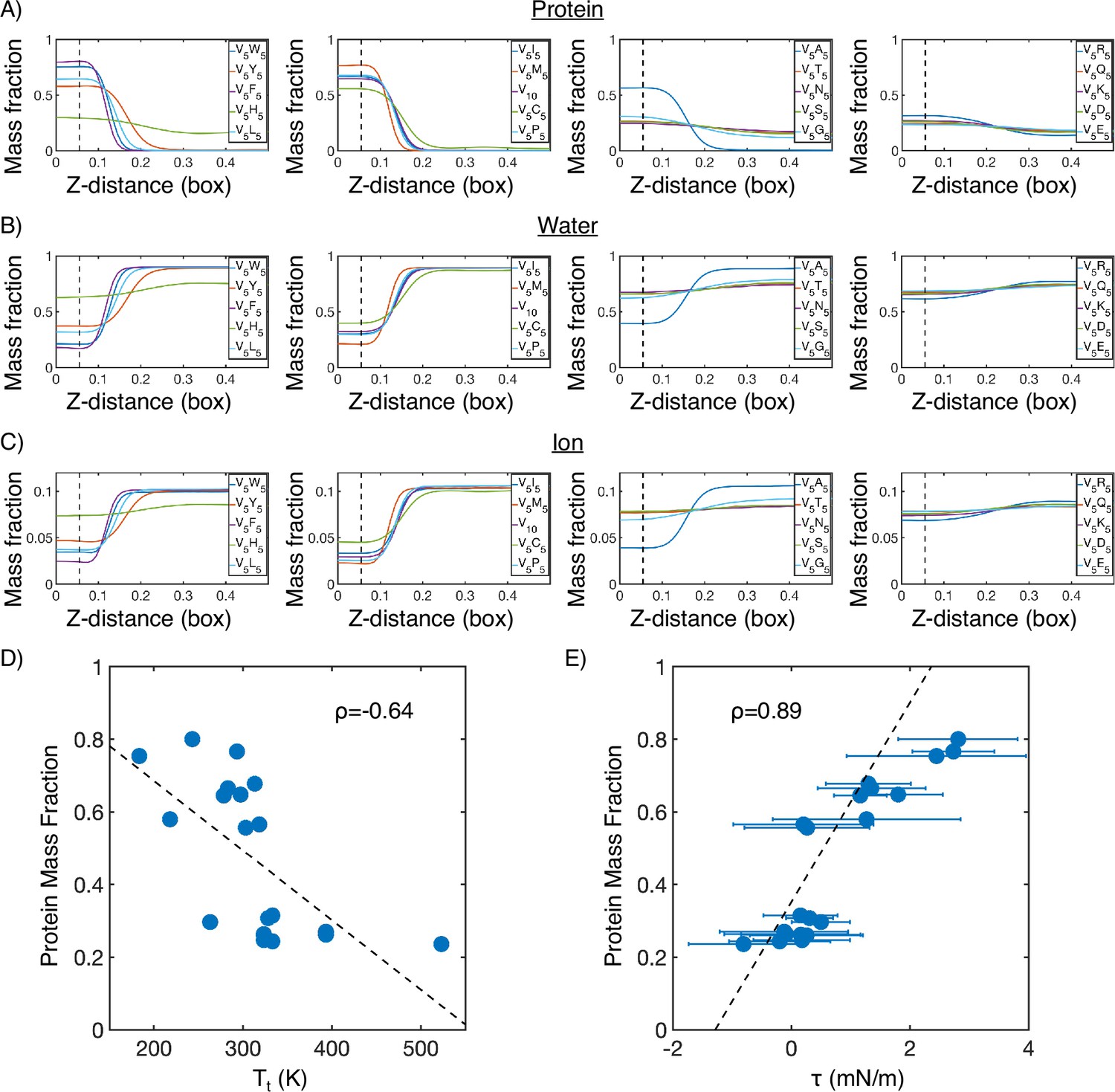
Mass fraction from MARTINI condensate simulations.
(A) Protein mass fraction along the Z-distance from the condensate center defined using the largest cluster. The Z-axis is defined as the direction perpendicular to the condensate-water interface. The dashed line represents a Z-distance of 0.06 box lengths. Average values below this threshold are used for correlation analysis in (D) and (E). (B) Water mass fraction along the Z-distance from the condensate center. (C) Ion mass fraction along the Z-distance from the condensate center. (D) Correlation between the average protein mass fraction and transition temperature () from Urry, 1997. ρ is the Pearson correlation coefficient between the two data sets, and the dashed diagonal line is the best fit line. Error bars represent SDs of the mean and are smaller than the symbols. (E) Correlation between the average protein mass fraction and the simulated surface tension (). is the Pearson correlation coefficient between the two data sets, and the dashed diagonal line is the best fit line. Error bars represent SDs of the mean taken over six equally spaced box length intervals.
Appendix 1—figure 2
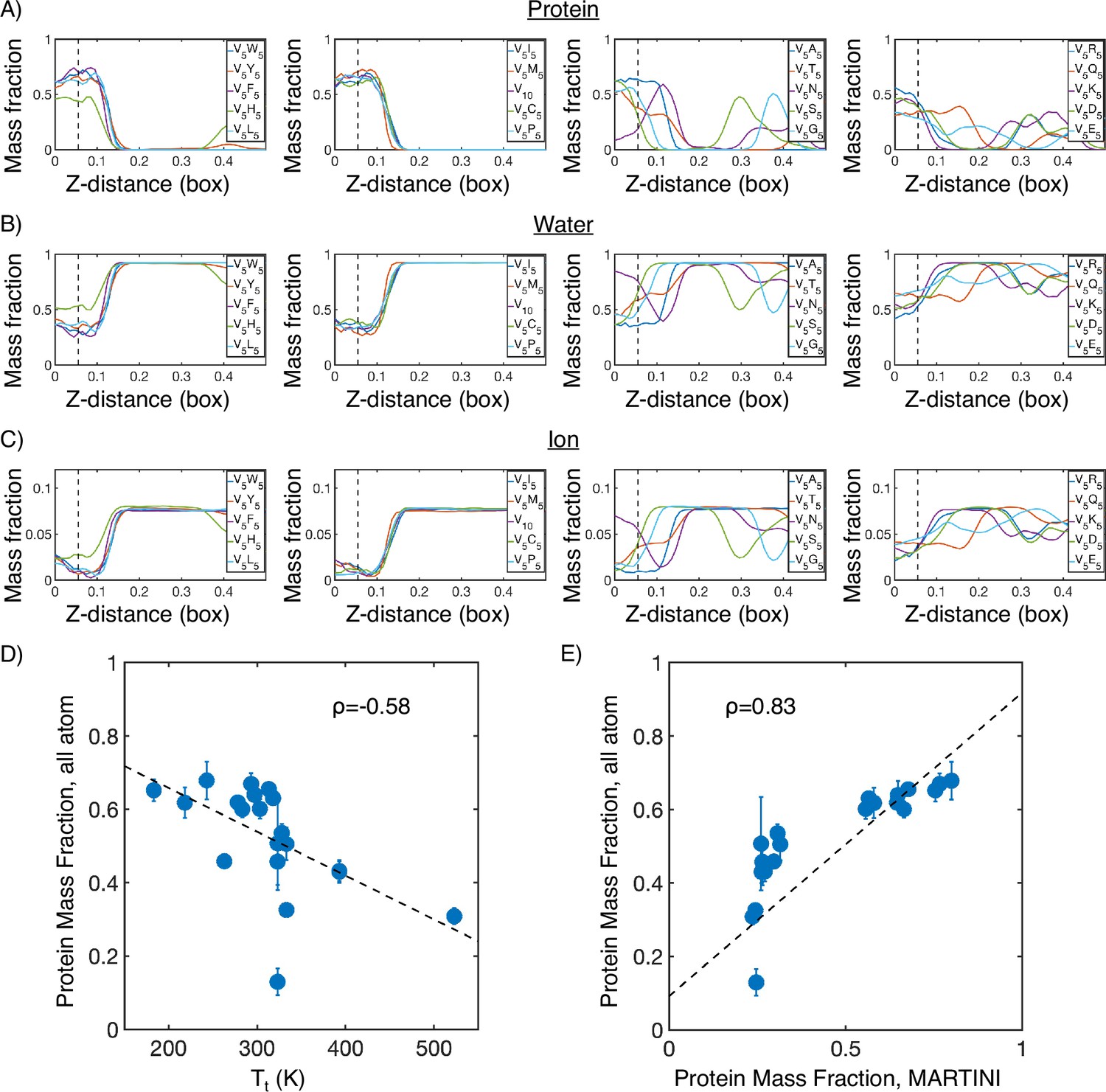
Mass fraction from atomistic condensate simulations.
(A) Protein mass fraction along the Z-distance from the condensate center defined using the largest cluster. The Z-axis is defined as the direction perpendicular to the condensate-water interface. The dashed line represents a Z-distance of 0.06 box lengths. Average values below this threshold are used for correlation analysis in (D) and (E). (B) Water mass fraction along the Z-distance from the condensate center. (C) Ion mass fraction along the Z-distance from the condensate center. (D) Correlation between the average protein mass fraction in all-atom simulations and transition temperature () from Urry, 1997. ρ is the Pearson correlation coefficient between the two data sets, and the dashed diagonal line is the best fit line. Error bars represent SDs of the mean taken over six equally spaced box length intervals. (E) Correlation between the average protein mass fraction from all-atom simulations and the average protein mass fraction from MARTINI simulations. is the Pearson correlation coefficient between the two data sets, and the dashed diagonal line is the best fit line. Error bars represent SDs of the mean taken over six equally spaced box length intervals.
Appendix 1—figure 3
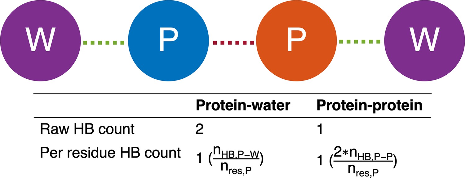
Graphical illustration of number of hydrogen bonds per protein residue.
The protein is depicted as blue and orange circles, and the water molecules are depicted as purple circles. Protein-protein and protein-water hydrogen bonds are drawn as red and green dashed lines, respectively. The number of protein-water hydrogen bonds per protein residue is calculated by taking the raw number of protein-water hydrogen bonds () and dividing by the number of residues in the protein (). Meanwhile, the number of protein-protein hydrogen bonds per protein residue is calculated by doubling the number of protein-protein hydrogen bonds () and dividing by the number of residues in the protein (). The extra factor of 2 accounts for the fact that, in the case of protein-protein hydrogen bonds, both the donor and the acceptor must reside within the protein.
Appendix 1—figure 4
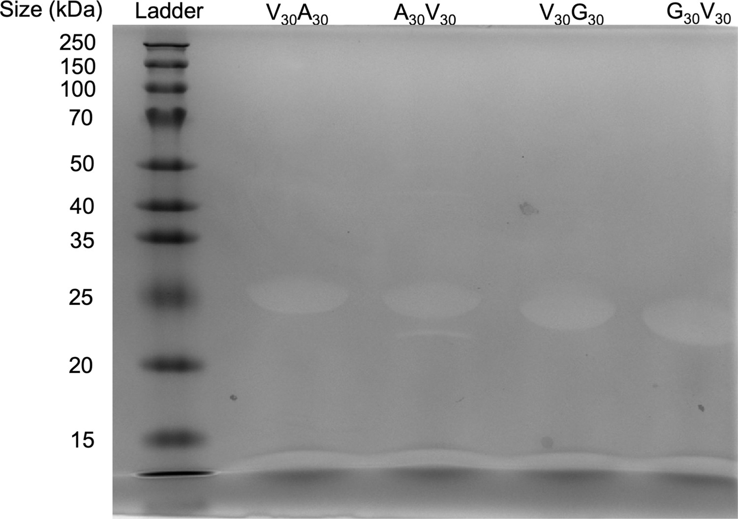
SDS-PAGE gel of elastin-like polypeptide (ELP).
The purity of the protein is >95%.
-
Appendix 1—figure 4—source data 1
Original files for western blot analysis displayed in Appendix 1—figure 4.
- https://cdn.elifesciences.org/articles/90750/elife-90750-app1-fig4-data1-v1.zip
-
Appendix 1—figure 4—source data 2
Original western blots for Appendix 1—figure 4, indicating the relevant bands and treatments.
- https://cdn.elifesciences.org/articles/90750/elife-90750-app1-fig4-data2-v1.zip
Appendix 1—figure 5
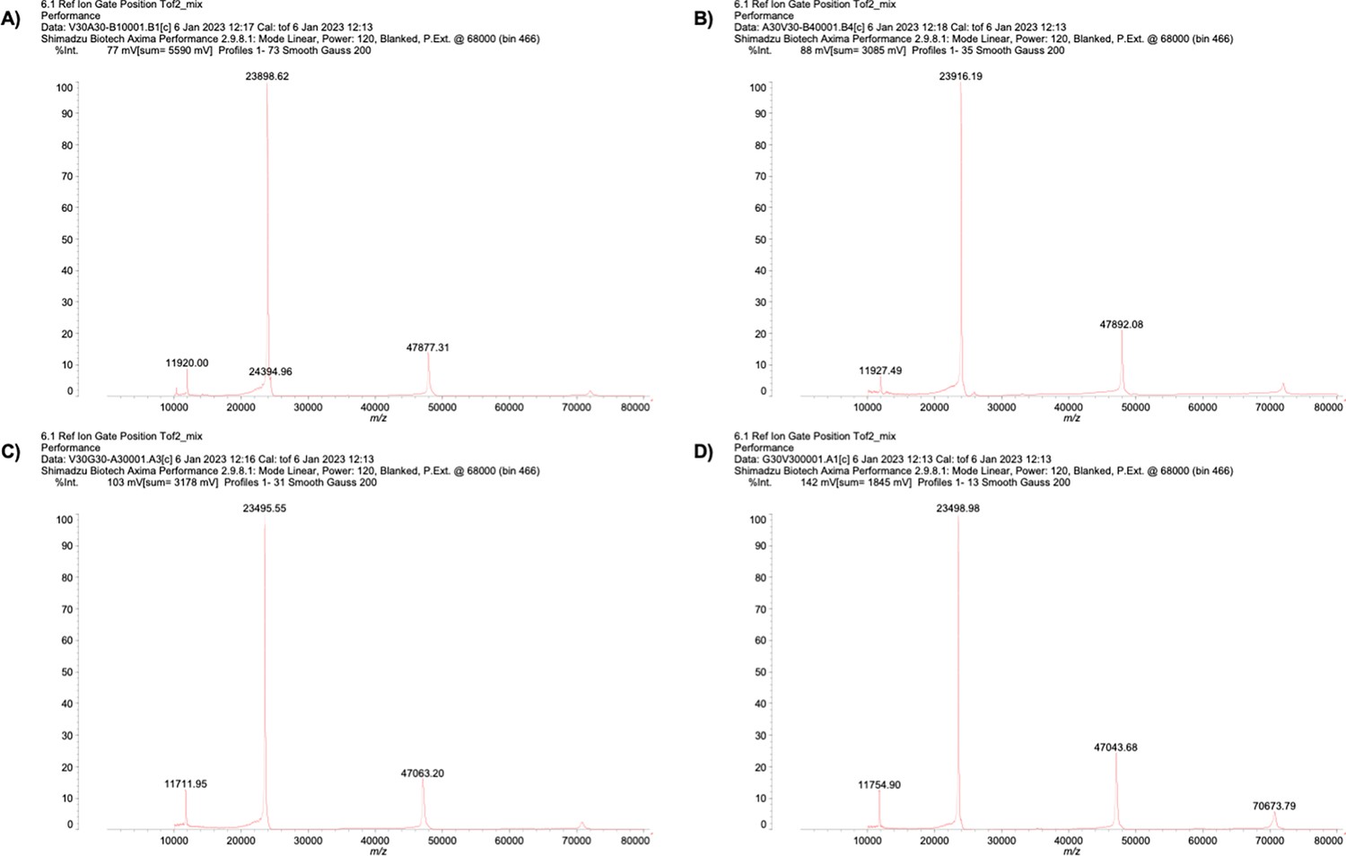
Mass spectrum of (A) V30A30, (B) A30V30, (C) V30G30, and (D) G30V30.
Appendix 1—figure 6
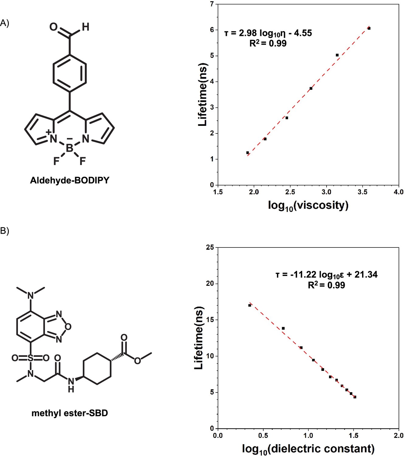
Calibration curves of fluorophores.
(A) Lifetime-viscosity calibration curve is quantified in the glycerol at different temperatures (10°C η = 3900 cP; 20°C η = 1,412 cP; 30°C η = 612 cP; 40°C η = 284 cP; 50°C η = 142 cP; 60°C η = 81.3 cP) Segur and Oberstar, 1951?. The fluorophore concentration is 5 μM. (B) Lifetime-dielectric constant calibration curve is quantified in the MeOH-1,4-dioxane mixture. , .
Tables
Appendix 1—table 1
Maximum allowed solvent-accessible surface area (SASA) for each amino acid, taken from Tien et al., 2013.
| Amino acid | Maximum SASA (Å2) |
|---|---|
| ALA | 129 |
| ARG | 274 |
| ASN | 195 |
| ASP | 193 |
| CYS | 167 |
| GLN | 225 |
| GLU | 223 |
| GLY | 104 |
| HIS | 224 |
| ILE | 197 |
| LEU | 201 |
| LYS | 236 |
| MET | 224 |
| PHE | 240 |
| PRO | 159 |
| SER | 155 |
| THR | 172 |
| TRP | 285 |
| TYR | 263 |
| VAL | 174 |
Appendix 1—table 2
Mass spectrum of purified ELP.
| Mass (Da) | ||
|---|---|---|
| Theoretical | MALDI-MS | |
| V30A30 | 24097.04 | 23898.62 |
| A30V30 | 24097.04 | 23916.19 |
| V30G30 | 23676.23 | 23495.55 |
| G30V30 | 23676.23 | 23498.98 |
Additional files
-
MDAR checklist
- https://cdn.elifesciences.org/articles/90750/elife-90750-mdarchecklist1-v1.pdf
-
Appendix 1—figure 4—source data 1
Original files for western blot analysis displayed in Appendix 1—figure 4.
- https://cdn.elifesciences.org/articles/90750/elife-90750-app1-fig4-data1-v1.zip
-
Appendix 1—figure 4—source data 2
Original western blots for Appendix 1—figure 4, indicating the relevant bands and treatments.
- https://cdn.elifesciences.org/articles/90750/elife-90750-app1-fig4-data2-v1.zip
Download links
A two-part list of links to download the article, or parts of the article, in various formats.
Downloads (link to download the article as PDF)
Open citations (links to open the citations from this article in various online reference manager services)
Cite this article (links to download the citations from this article in formats compatible with various reference manager tools)
Microphase separation produces interfacial environment within diblock biomolecular condensates
eLife 12:RP90750.
https://doi.org/10.7554/eLife.90750.4


