Optimal transport for automatic alignment of untargeted metabolomic data
- Nutrition and Metabolism Branch, International Agency for Research on Cancer, France
- Massachusetts Institute of Technology, Department of Mathematics, United States
Figures
Figure 1
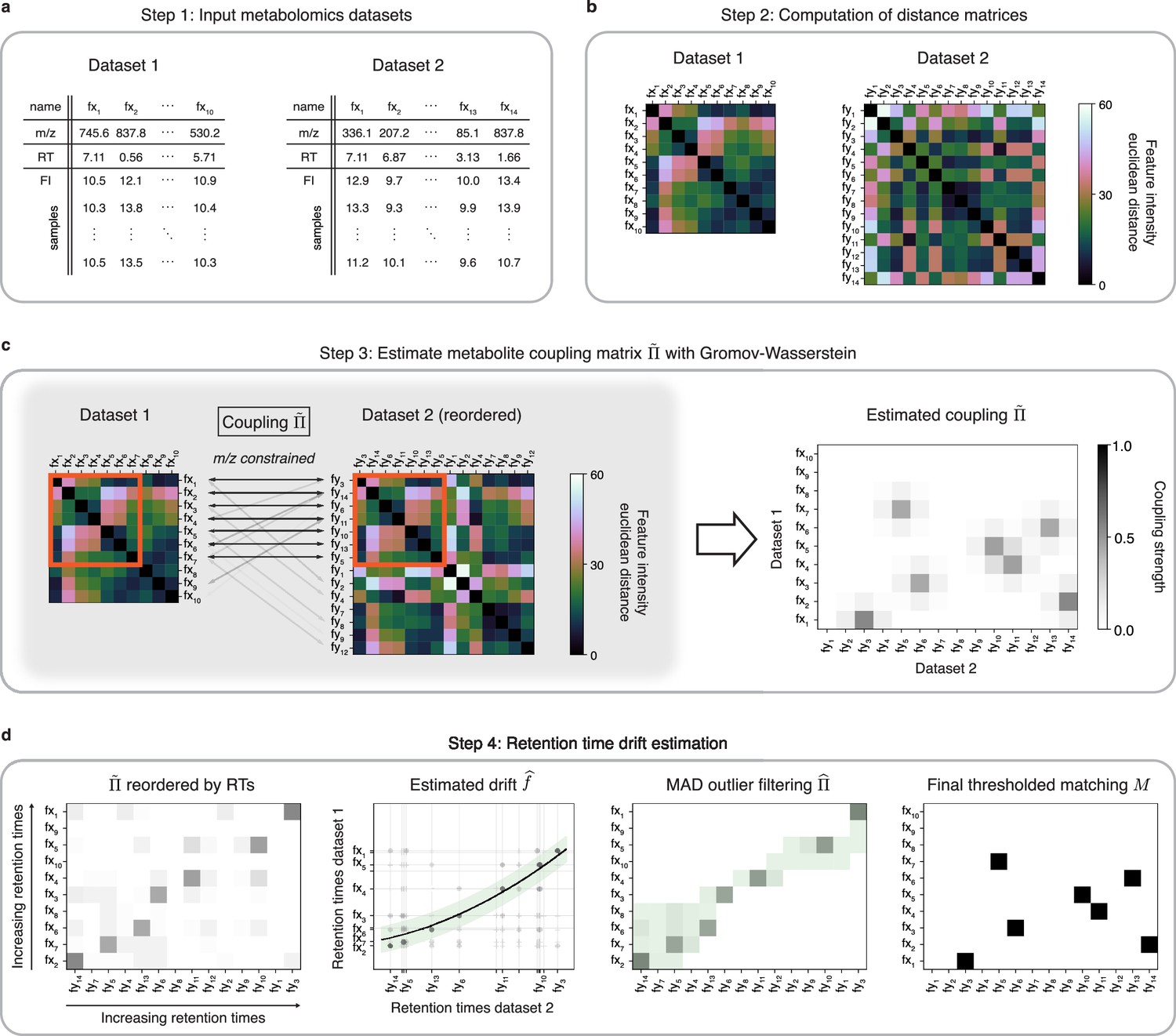
An optimal transport approach for combining untargeted metabolomics datasets (GromovMatcher).
(a) Inputs are two LC-MS datasets of unlabeled metabolic features (rows) identified by their , RT, and feature intensities across biospecimen samples. Both studies can have differing numbers of metabolic features and samples. (b) In both datasets, the intensities across samples of each metabolic feature are formed into a vector and Euclidean distances between these feature vectors are computed and stored in a distance matrix. (c) Based on the technique of optimal transport, the unbalanced GW algorithm learns a coupling matrix that places large weights when and likely correspond to the same metabolic feature. It optimizes to match features with similar pairwise distances (red outlined boxes) whose ratios are close. (d) The final step of GromovMatcher plots the retention times of features from both datasets against each other and fits a spline interpolation weighted by the estimated coupling weights . This retention time drift function is then used to set all entries to zero for those outlier pairs which exceed twice the median absolute deviation (MAD) around (green highlighted region). Finally, the coupling matrix is filtered and/or thresholded to obtain a refined coupling which is then binarized to obtain a one-to-one matching between a subset of metabolite pairs in both datasets.
Figure 2
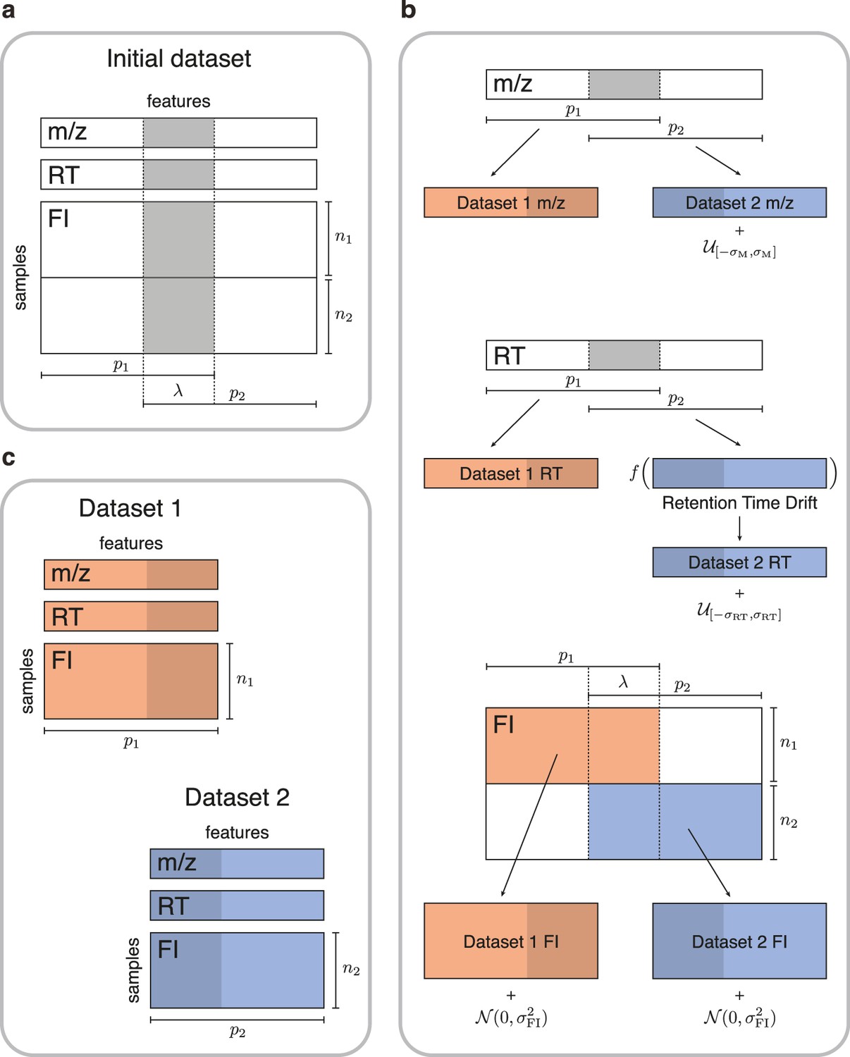
Simulated data for testing untargeted metabolomics alignment methods.
(a) Initial LC-MS dataset taken from the EXPOsOMICS project with , RT, and feature intensities of metabolites identified in cord blood across newborns. (b) Newborns (rows) are split into two disjoint groups of sizes and respectively and metabolic features (columns) are split into two equal groups of size with overlap where (Materials and methods). Datasets are perturbed by additive noise of magnitude and a nonlinear drift is applied to the RTs of dataset 2. (c) The two resulting datasets share , or 75% of the original dataset’s metabolic features.
Figure 3 with 2 supplements
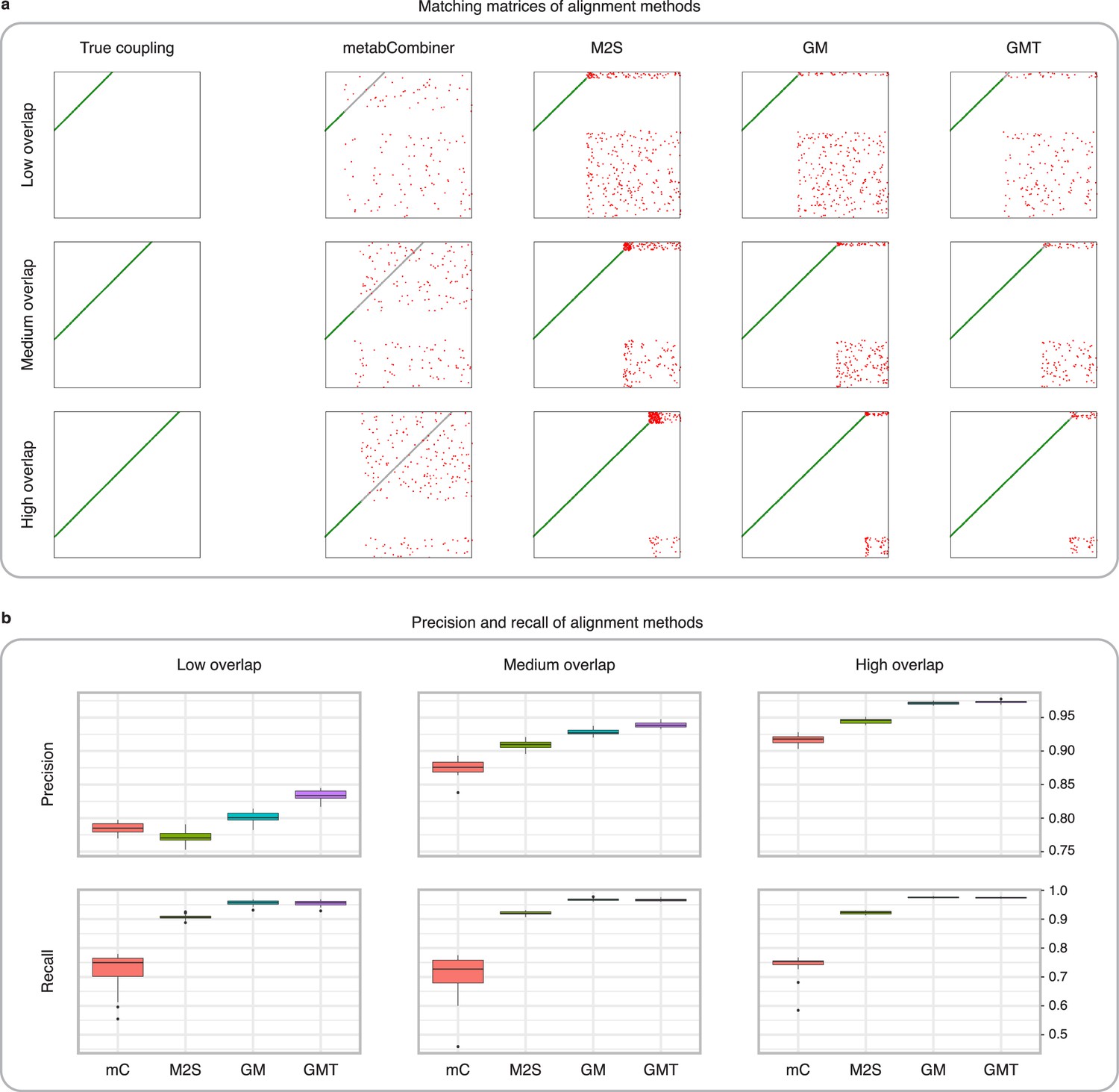
Comparison of MetabCombiner, M2S, and GromovMatcher on simulated data.
(a) Ground-truth matchings, and matchings inferred by metabCombiner, M2S, GM, and GMT. Pairs of datasets are generated for three levels of overlap (low, medium and high), with a medium noise level (Materials and methods). Matches correctly recovered (true positives) are represented in green. True matches that are not recovered (false negatives) are highlighted in grey. Incorrect matches (false positives) are plotted in red. Features in rows and columns of matching matrices are reordered for visual clarity. (b) Average precision and recall on 20 randomly generated pairs of datasets, for three levels of overlap (low, medium, and high) with a medium noise level.
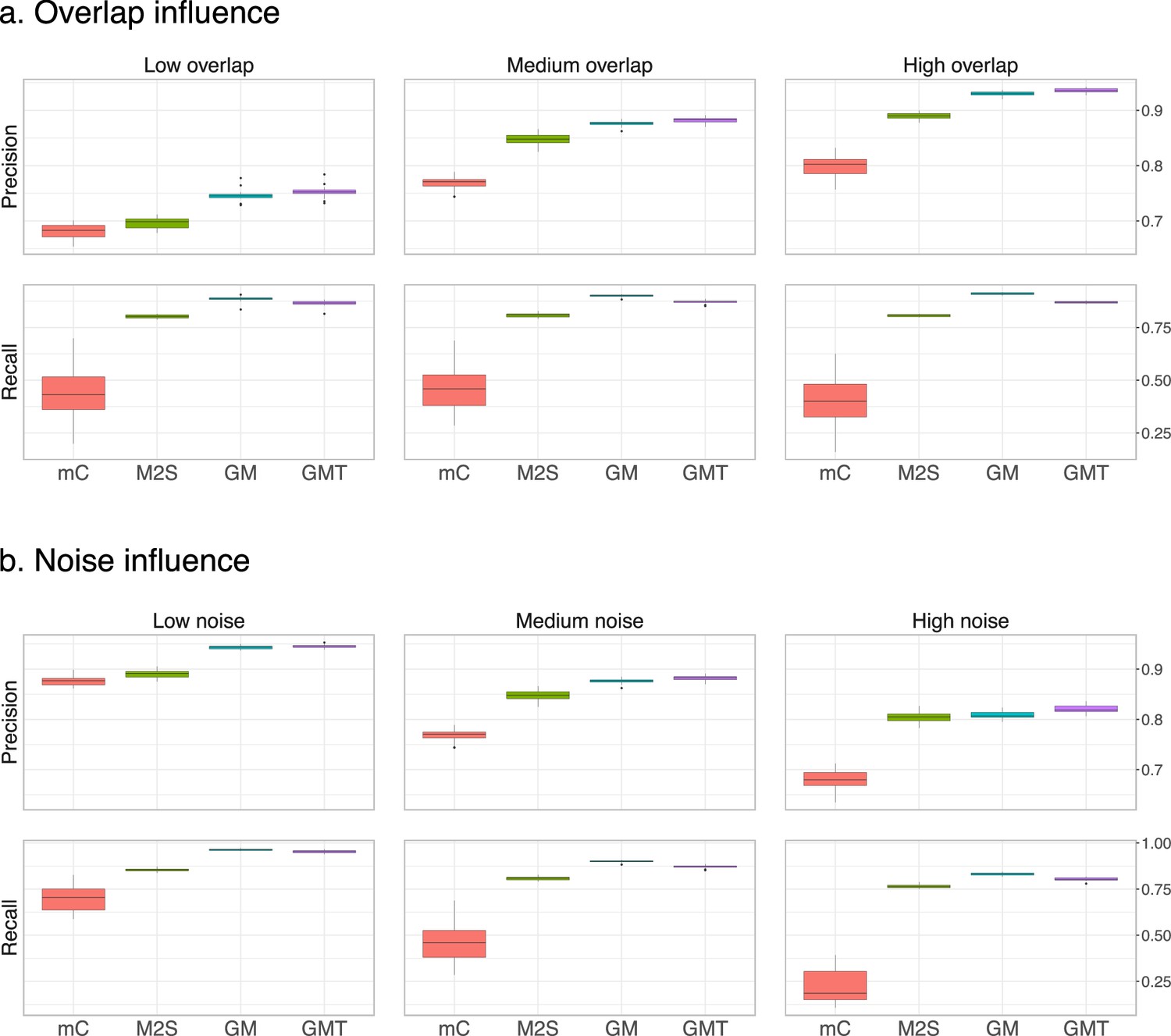
Figure 3—figure supplement 1
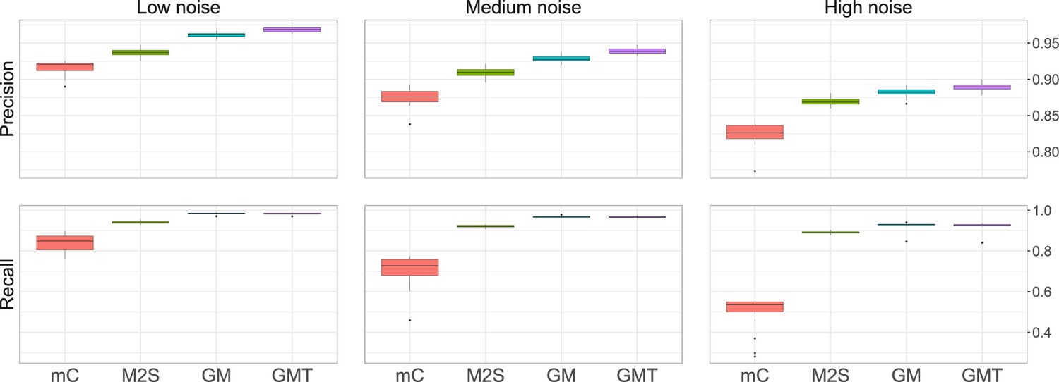
Average precision and recall obtained on simulated data, with fixed overlap .
The noise level corresponds to different values of and . High, medium, and low noise level correspond to and (1, 1) respectively. We run 20 simulations for each setting.
Figure 3—figure supplement 2
Performance on centered and scaled data.
The feature intensities of both datasets are centered and scaled to have means of 0 and standard deviations of 1. The average precision and recall of the three methods are computed on 20 randomly generated pairs of datasets, for (a) three levels of overlap (low, medium and high corresponding to and 0.75, respectively) with a medium noise level (), and (b) fixed medium overlap () and three different noise levels (low, medium and high corresponding to and (1, 1) respectively).
Figure 4 with 3 supplements
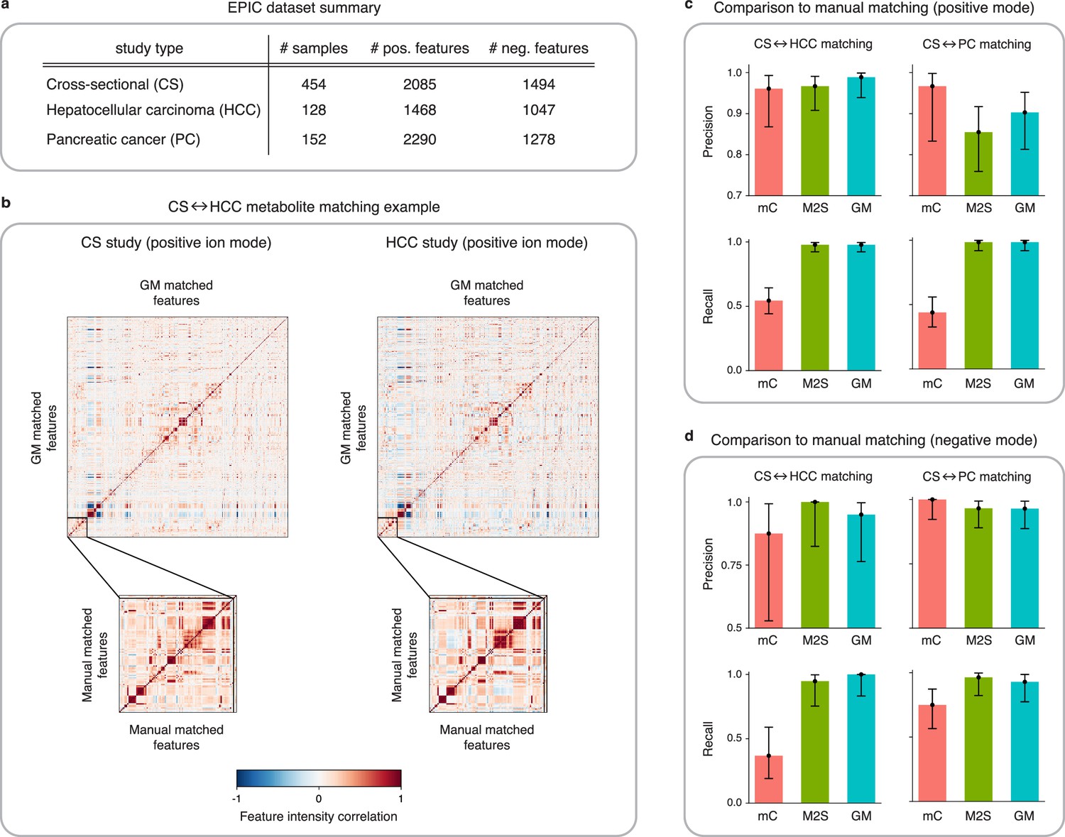
Application of GromovMatcher and comparison to existing methods on EPIC dataset.
(a) Dimensions of the three EPIC studies used. For each ionization mode, the cross-sectional (CS) study is aligned successively with the hepatocellular carcinoma (HCC) study and the pancreatic cancer (PC) study. (b) Demonstration of expert manual matching and GromovMatcher (GM) matching between the CS and HCC studies in positive mode. Experts manually match 90 features (Table 1) from Loftfield et al., 2021 and the correlation matrices of these features in both datasets have similar structure (bottom two matrices). GM discovers 996 shared features between the CS and HCC datasets which have similar correlation structure (top two matrices). We validate that 88 of the 90 features from the manually expert matched subset are contained in the set of features matched by GM. (c) Performance of metabCombiner (mC), M2S and GM in positive mode. Precisions and recalls are measured on a validation subset of 163 manually examined features, and 95% confidence intervals are computed using modified Wilson score intervals. (d) Performance of mC, M2S, and GM in negative mode. Precision and recall are measured on a validation subset of 42 manually examined features, and 95% confidence intervals are computed using modified Wilson score intervals. See Table 2 and Table 3 for exact precisions, recalls, and confidence intervals in positive and negative mode, respectively.
Figure 4—figure supplement 1
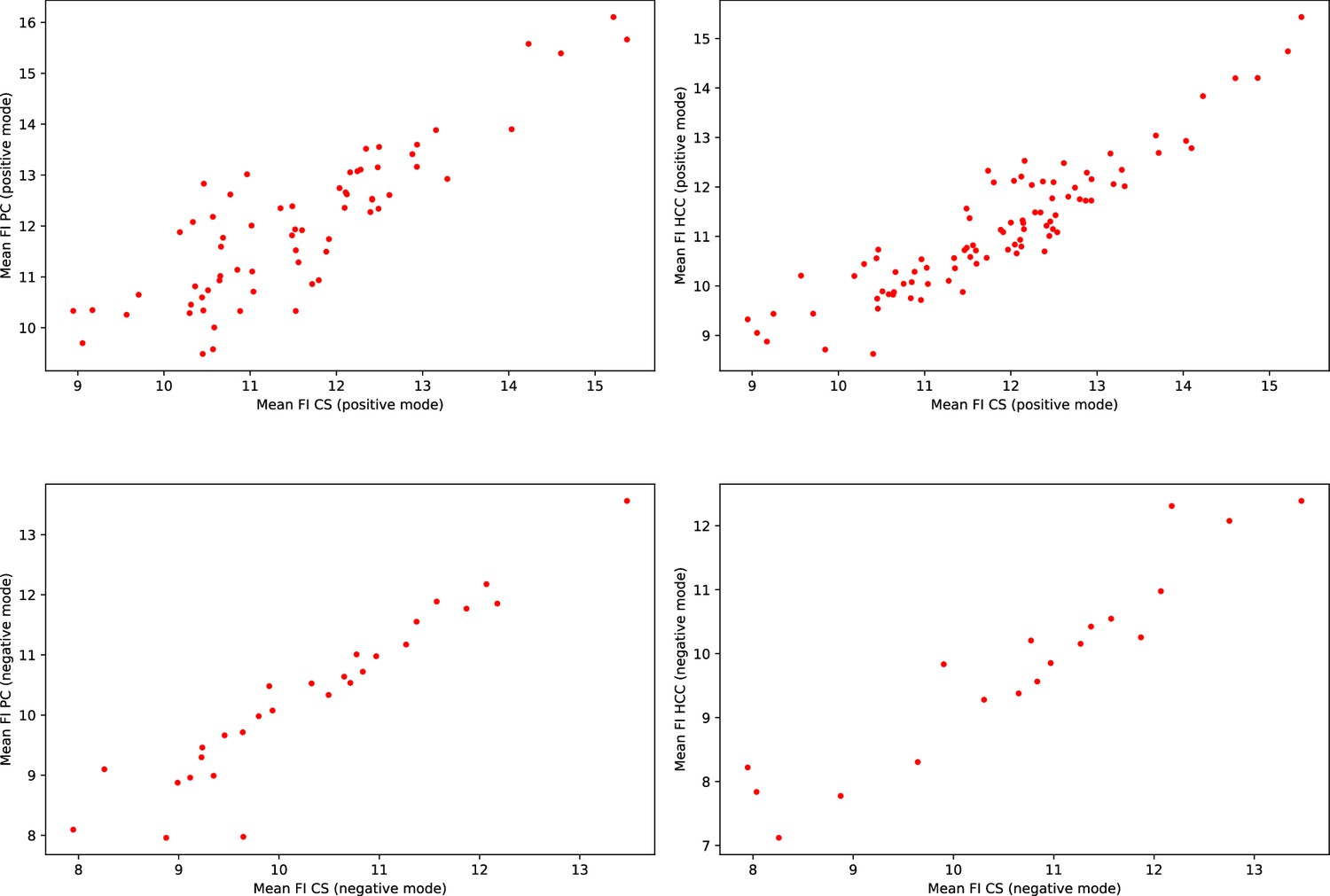
Consistency of the mean feature intensities (FI) in EPIC.
Each scatter plot represents the mean feature intensities of manually matched features from the validation subset. Each dot represents a pair of manually matched features. The axis represent the mean feature intensities recorded in the two different studies.
Figure 4—figure supplement 2
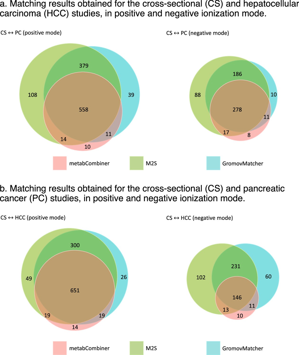
Overlap between the matching results obtained by metabCombiner, M2S and GromovMatcher in EPIC.
Venn diagrams are not up to scale.
Figure 4—figure supplement 3
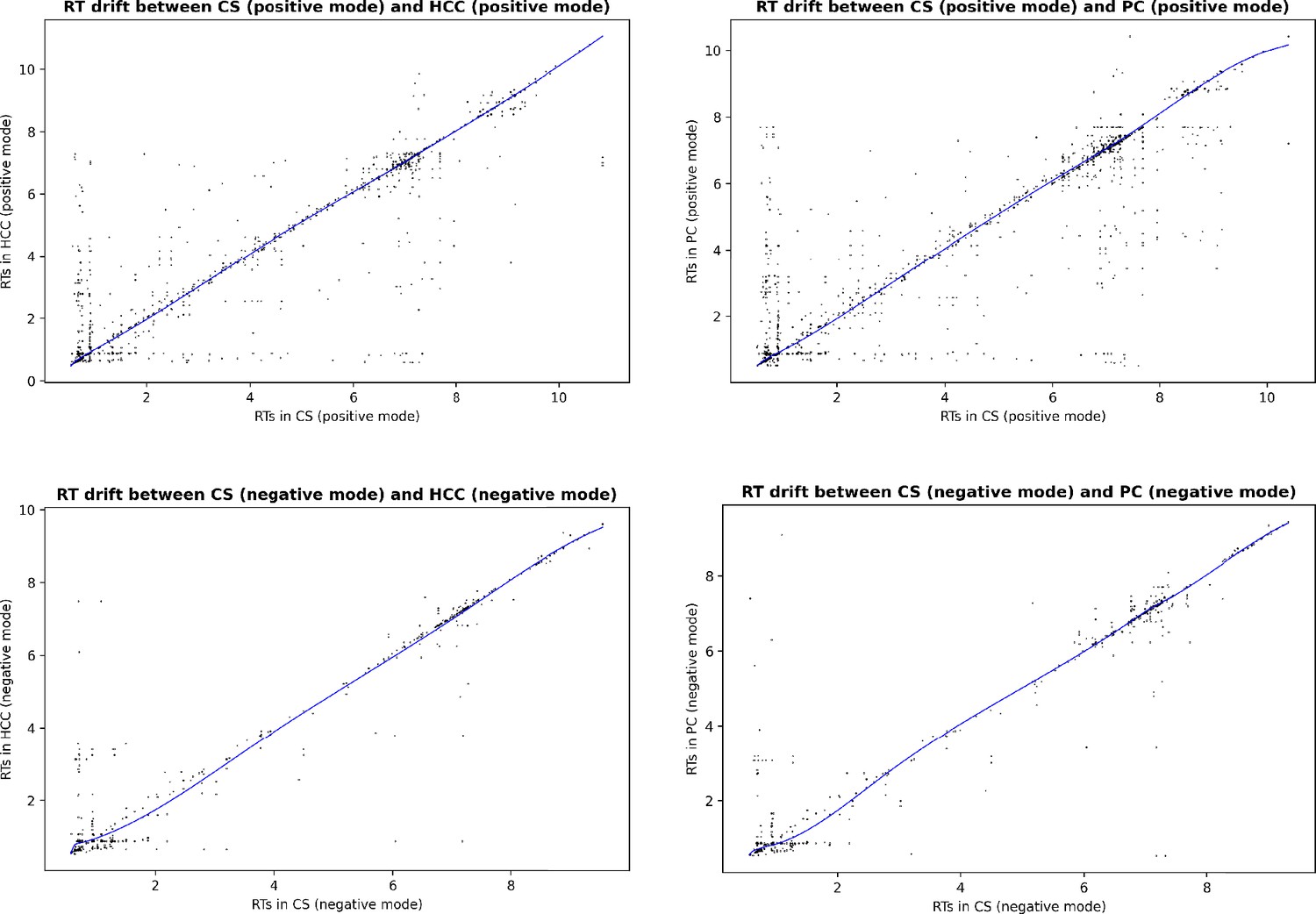
Estimated RT drift between the EPIC studies aligned in the main experiment.
Each dot correspond to a candidate matched pair after the first step of GM ( constrained GW matching), before the RT drift estimation and RT-based filtering.
Figure 5
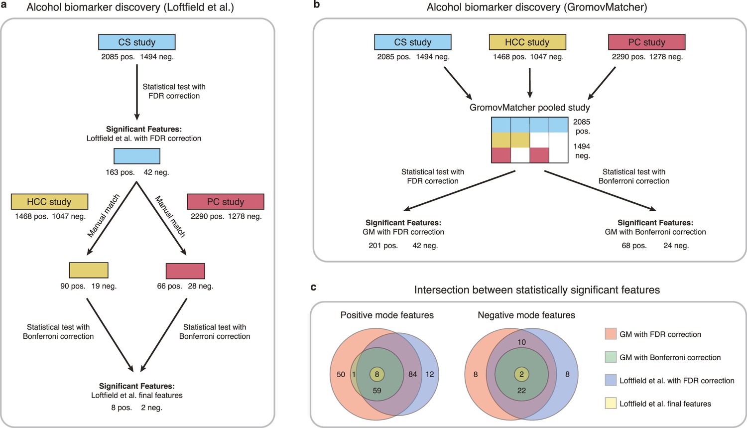
Comparison of GromovMatcher and Loftfield et al., 2021 analysis for alcohol biomarker discovery on EPIC data.
(a) Loftfield study implemented a discovery step, examining the relationship between alcohol intake and metabolic features in the CS study. The significant features in CS were manually matched to features from the HCC and PC and the analysis was repeated using samples from the HCC and PC studies. After this step, 10 features associated with alcohol intake were identified. (b) GromovMatcher analysis begins by matching features from CS study to HCC and PC studies respectively (top blue, yellow, and red boxes). Samples corresponding to each CS feature are combined with the samples of its matched feature in the HCC study, PC study, or both. This generates a larger pooled data matrix with the same number of features as the CS study but with more samples pooled across the three original studies (center matrix). Because some features in the CS study may not have matches in HCC or PC, the corresponding entries in the pooled matrix are set to NaN/missing values (white regions in matrix). Each column/feature in this matrix is statistically tested for association with alcohol intake (ignoring missing values) and an FDR or a stricter Bonferroni correction is performed to retain only a subset of features from the pooled study that have a strong association. (c) Venn diagrams show intersection of feature sets (in positive and negative mode) found to be associated with alcohol intake by one of the four different analyses.
Appendix 2—figure 1
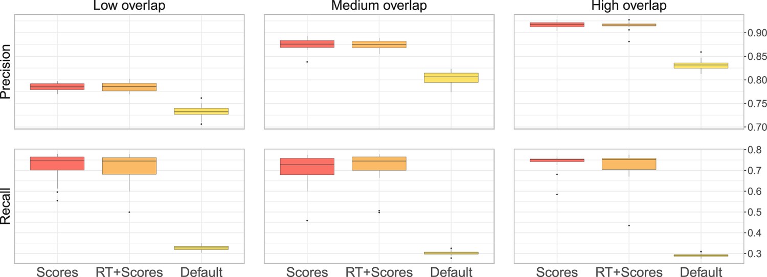
Performance of metabCombiner with the different parameter settings.
The first setting, labelled ‘Scores’ correspond to the design of our main analysis, where 100 randomly selected true pairs are supplied to metabCombiner to set the scoring weights automatically, but are not otherwise used. In the second setting, labelled ‘Scores + RT’, metabCombiner is allowed to use the 100 true pairs not only to set the scoring weights, but also to estimate the RT drift. Finally, in the third ‘Default’ setting, we do not use any prior knowledge for the RT drift estimation and keep the scoring weights’ default values.
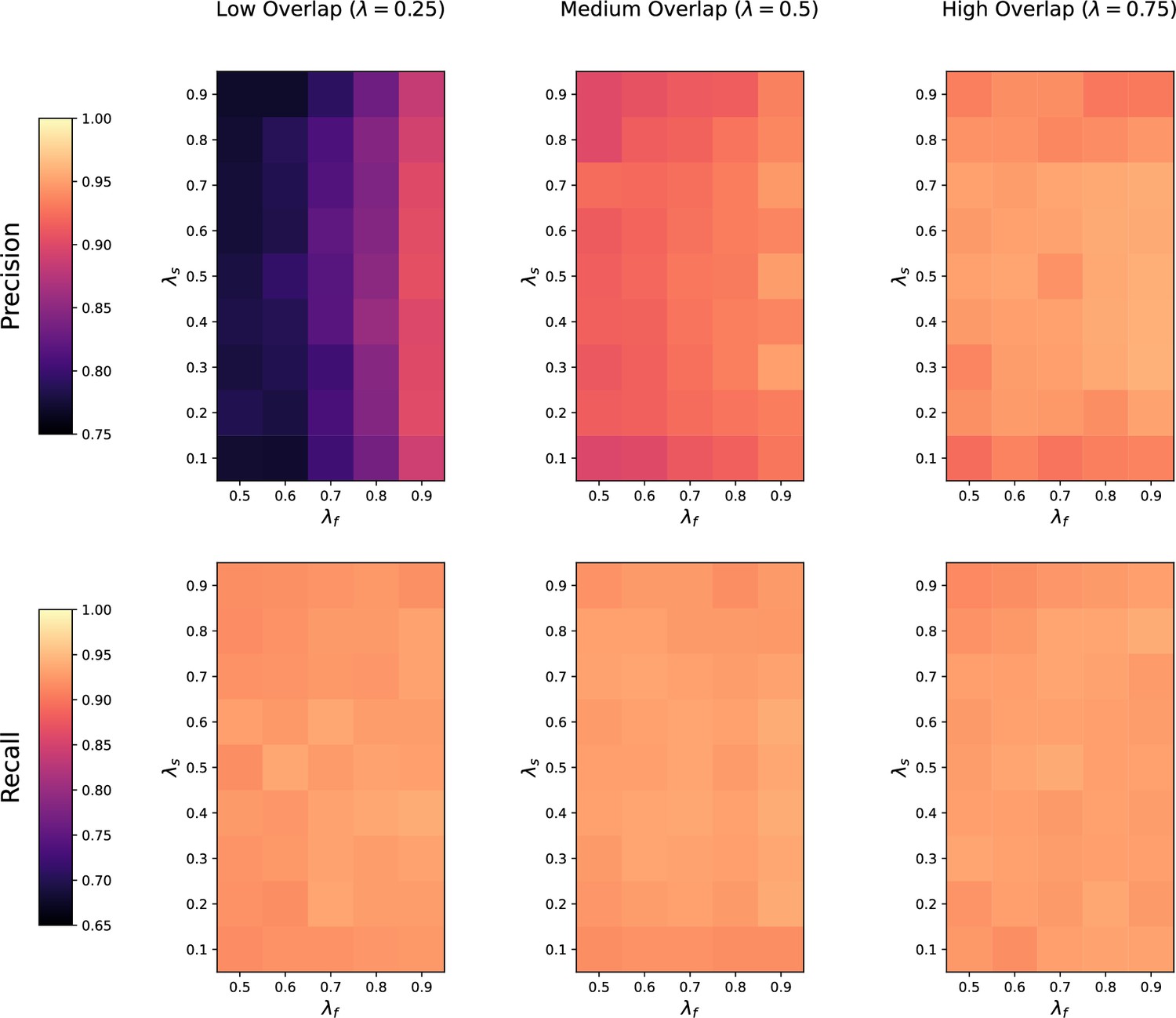
Appendix 3—figure 1
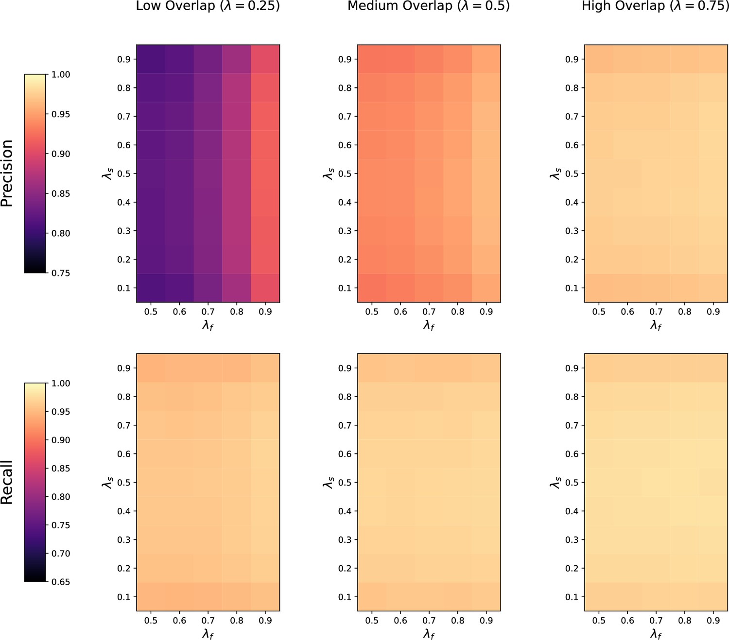
Sensitivity of thresholded GromovMatcher (GMT) to feature overlap fraction , feature imbalance fraction , and sample imbalance fraction between two datasets being matched.
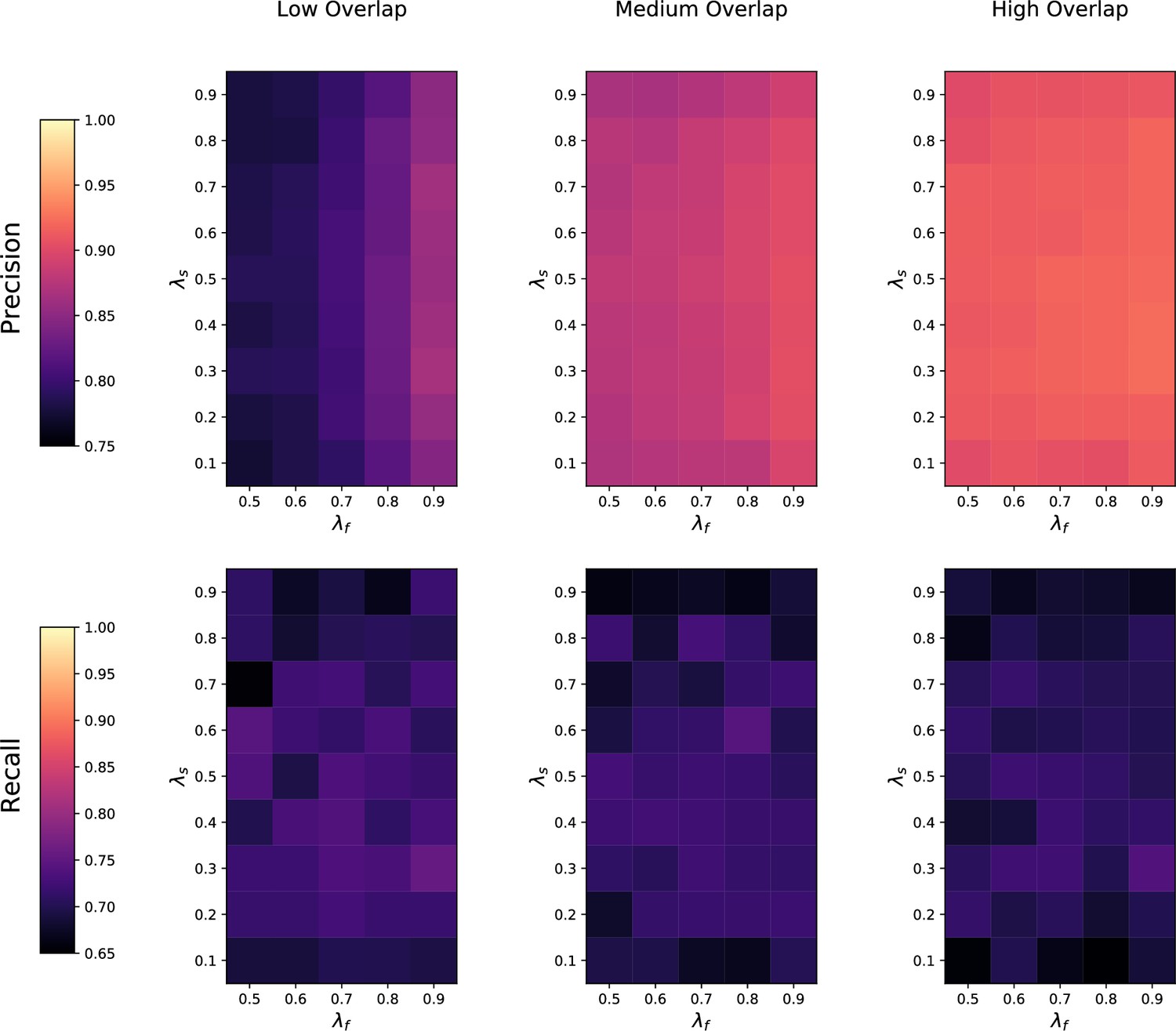
Appendix 3—figure 2
Sensitivity of M2S to feature overlap fraction , feature imbalance fraction , and sample imbalance fraction between two datasets being matched.
Appendix 3—figure 3
Sensitivity of metabCombiner (mC) to feature overlap fraction , feature imbalance fraction , and sample imbalance fraction between two datasets being matched.
Appendix 5—figure 1

Overlap between the 706 features common to the HCC and PC studies found via reference matching, and the 938 features common to HCC and PC found by direct matching.
Appendix 5—figure 2

Overlap between the features identified as common to the three EPIC studies using either the CS study or the HCC study as a reference.
Tables
Table 1
Results from the manual matching conducted for Loftfield et al., 2021.
Features from the CS study (163 features in positive mode, 42 features in negative mode) were manually investigated for matches in the HCC and PC studies.
| Study | Manual matches found in positive mode | Manual matches found in negative mode |
|---|---|---|
| Hepatocellular carcinoma (HCC) | 90 | 19 |
| Pancreatic cancer (PC) | 66 | 28 |
Table 2
Precision and recall on the EPIC validation subset in positive mode.
95% confidence intervals were computed using modified Wilson score intervals (Brown et al., 2001; Agresti and Coull, 1998).
| Method | Precision | Recall | Precision | Recall |
| GromovMatcher | 0.989 (0.939, 0.999) | 0.978 (0.923, 0.996) | 0.903 (0.813, 0.952) | 0.985 (0.919, 0.999) |
| M2S | 0.967 (0.908, 0.991) | 0.978 (0.923, 0.996) | 0.855 (0.759, 0.917) | 0.985 (0.919, 0.999) |
| metabCombiner | 0.961 (0.868, 0.993) | 0.544 (0.442, 0.643) | 0.967 (0.833, 0.998) | 0.439 (0.326, 0.559) |
Table 3
Precision and recall on the EPIC validation subset in negative mode.
95% confidence intervals were computed using modified Wilson score intervals (Brown et al., 2001; Agresti and Coull, 1998).
| Method | Precision | Recall | Precision | Recall |
| GromovMatcher | 0.950 (0.764, 0.997) | 1.000 (0.832, 1.000) | 0.929 (0.774, 0.987) | 0.929 (0.774, 0.987) |
| M2S | 1.000 (0.824, 1.000) | 0.947 (0.754, 0.997) | 0.931 (0.780, 0.988) | 0.964 (0.823, 0.998) |
| metabCombiner | 0.875 (0.529, 0.993) | 0.368 (0.191, 0.590) | 1.000 (0.845, 1.000) | 0.750 (0.566, 0.873) |
Appendix 2—table 1
Performance of M2S in a setting where the RT drift between studies is linear.
| Metric | Low overlap | Medium overlap | High overlap |
|---|---|---|---|
| Precision | 0.831 | 0.917 | 0.947 |
| Recall | 0.934 | 0.933 | 0.939 |
Appendix 4—table 1
Precision and recall on the EPIC validation subset for unnormalized data in (a) positive mode, and (b) negative mode.
95% confidence intervals were computed using modified Wilson score intervals Brown et al., 2001; Agresti and Coull, 1998.
| Method | Precision | Recall | Precision | Recall |
| GromovMatcher | 0.988 (0.937, 0.999) | 0.944 (0.876, 0.997) | 0.873 (0.776, 0.932) | 0.939 (0.854, 0.976) |
| M2S | 0.967 (0.908, 0.991) | 0.978 (0.923, 0.996) | 0.855 (0.759, 0.917) | 0.985 (0.919, 0.999) |
| metabCombiner | 0.979 (0.889, 0.999) | 0.511 (0.410, 0.612) | 0.926 (0.766, 0.987) | 0.379 (0.271, 0.499) |
| (a) Positive mode | ||||
| Method | Precision | Recall | Precision | Recall |
| GromovMatcher | 0.950 (0.764, 0.997) | 1.000 (0.832, 1.000) | 0.964 (0.823, 0.998) | 0.964 (0.823, 0.998) |
| M2S | 1.000 (0.824, 1.000) | 0.947 (0.754, 0.997) | 0.931 (0.780, 0.988) | 0.964 (0.823, 0.998) |
| metabCombiner | 1.000 (0.566, 1.000) | 0.263 (0.118, 0.488) | 1.000 (0.785, 1.000) | 0.500 (0.326, 0.674) |
| (b) Negative mode | ||||
Additional files
Download links
A two-part list of links to download the article, or parts of the article, in various formats.
Downloads (link to download the article as PDF)
Open citations (links to open the citations from this article in various online reference manager services)
Cite this article (links to download the citations from this article in formats compatible with various reference manager tools)
Optimal transport for automatic alignment of untargeted metabolomic data
eLife 12:RP91597.
https://doi.org/10.7554/eLife.91597.3


