Machine learning and biological validation identify sphingolipids as potential mediators of paclitaxel-induced neuropathy in cancer patients
- Institute of Clinical Pharmacology, Goethe - University, Germany
- Fraunhofer Institute for Translational Medicine and Pharmacology ITMP, and Fraunhofer Cluster of Excellence for Immune Mediated Diseases CIMD, Germany
- Goethe University, Department of Gynecology and Obstetrics, Germany
- German Cancer Consortium (DKTK) and German Cancer Research Center (DKFZ), Germany
- Goethe University, University Cancer Center Frankfurt (UCT), Goethe University Hospital, Germany
- Oncology Center, Sana-Klinikum Offenbach, Germany
Figures
Figure 1
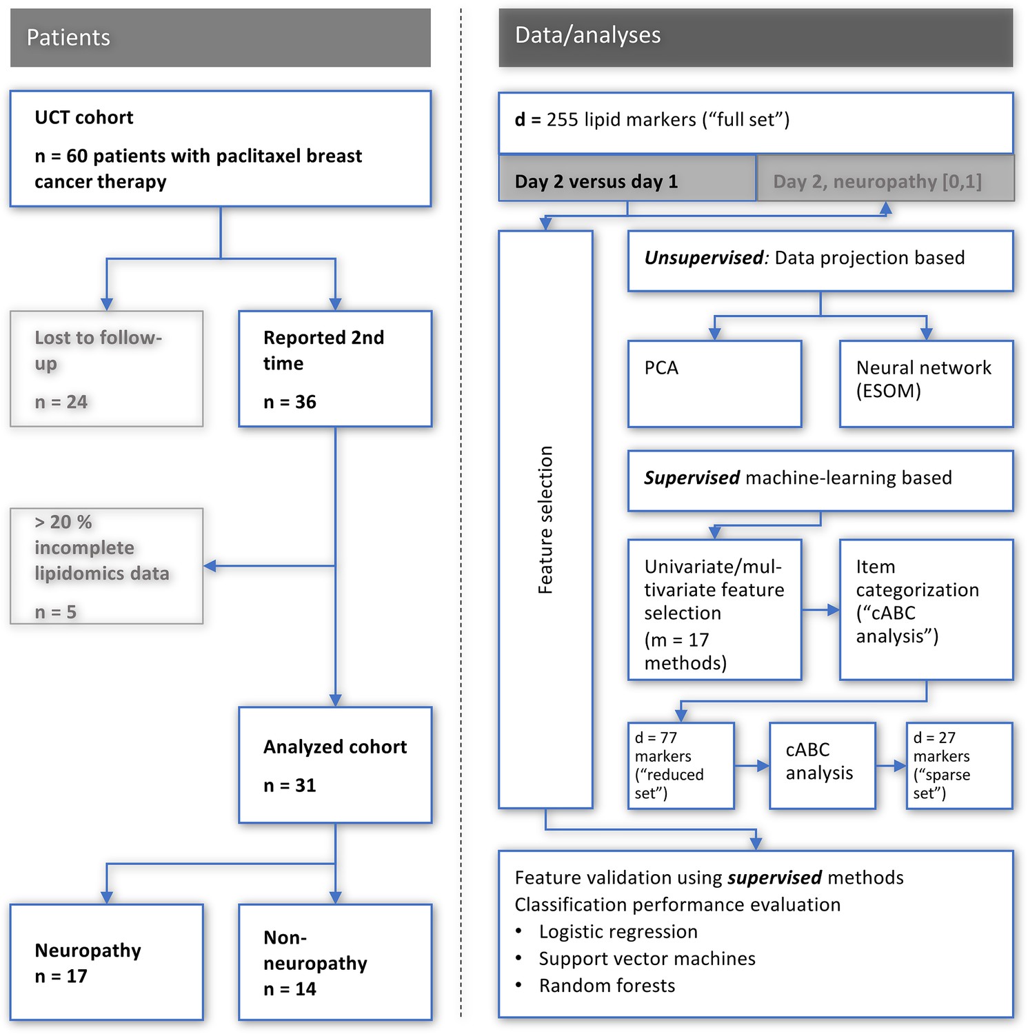
Flowchart showing the number of patients included and the workflow of the data analysis.
UCT: University Cancer Center Frankfurt, PCA: principal component analysis, ESO: emergent self-organizing maps, cABC analysis: computed ABC analysis. The figure was created using Microsoft PowerPoint (Redmond, WA, USA) on Microsoft Windows 11 running in a virtual machine powered by VirtualBox 6.1.36 (Oracle Corporation, Austin, TX, USA) as guest on Linux, and then further modified with the free vector graphics editor “Inkscape version 1.2 for Linux, https://inkscape.org/.
Figure 2 with 1 supplement
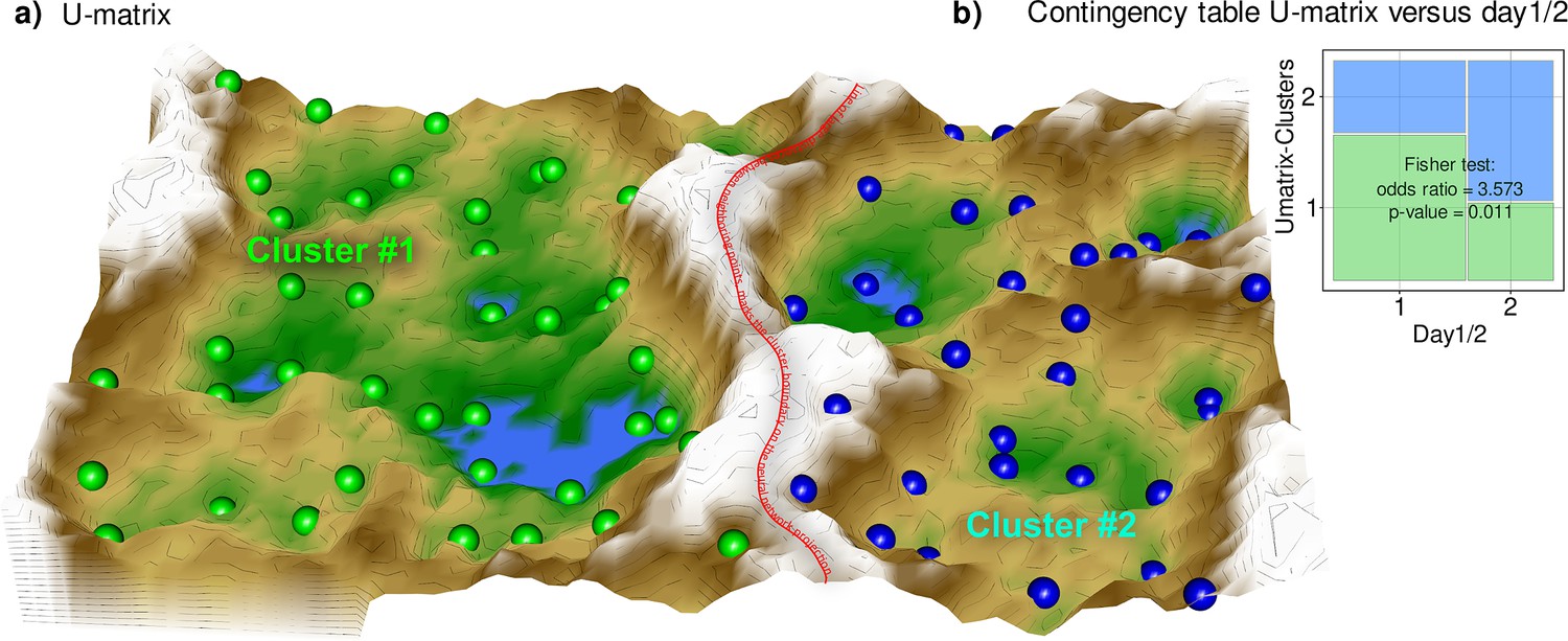
Results of a projection of the z-standardized log-transformed lipidomics data onto a lower-dimensional space by means of a self-organizing map of artificial neurons (bottom).
(a) 3D display of an emergent self-organizing map (ESOM), providing a three-dimensional U-matrix visualization (Thrun et al., 2016) of distance-based structures of the serum concentrations of d=255 lipid mediators following projection of the data points onto a toroid grid of 4000 neurons where opposite edges are connected. The dots represent the so-called ‘best matching units’ (BMU), that is neurons on the grid that after ESOM learning carried a data vector that was most similar to a data vector of a sample in the data set. Only those neurons of the originally 4000 neurons are shown that carried vectors of cases from the present data set. Please also note that one BMU can carry vectors of several cases, that is the number of BMUs is not necessarily equal to the number of cases. A cluster structure emerges from visualization of the distances between neurons in the high-dimensional space by means of a U-matrix (Izenmann, 2009). The U-matrix was colored as a geographical map with brown or snow-covered heights and green valleys with blue lakes, symbolizing high or low distances, respectively, between neurons in the high-dimensional space. Thus, valleys left and right of the ‘mountain range’ in the middle indicate clusters and watersheds, that is the line of large distances between neighboring points, indicate borderlines between different clusters. Tat is, the mountain range with ‘snow-covered’ heights separates main clusters according to probe acquisition at day 1 or day 2, that is before and after treatment with paclitaxel. BMUs belonging to the two different clusters are colored green or bluish. (b) Mosaic plot of the prior classes (day 1 or day 2) versus the ESOM/Umatrix based clusters. The separation corresponded to the previous classification into pre- and post-therapy probes (day1/2). Cluster #1 was composed of more probes taken on day #1, while probes from day 2 were overrepresented in cluster #2. The figure has been created using the R software package (version 4.1.2 for Linux; https://CRAN.R-project.org/ R Development Core Team, 2008), R library ‘ggplot2’ (https://cran.r-project.org/package=ggplot2 (94)) and our R package ‘Umatrix’ (https://cran.r-project.org/package=Umatrix Lötsch et al., 2018a).
Figure 2—figure supplement 1
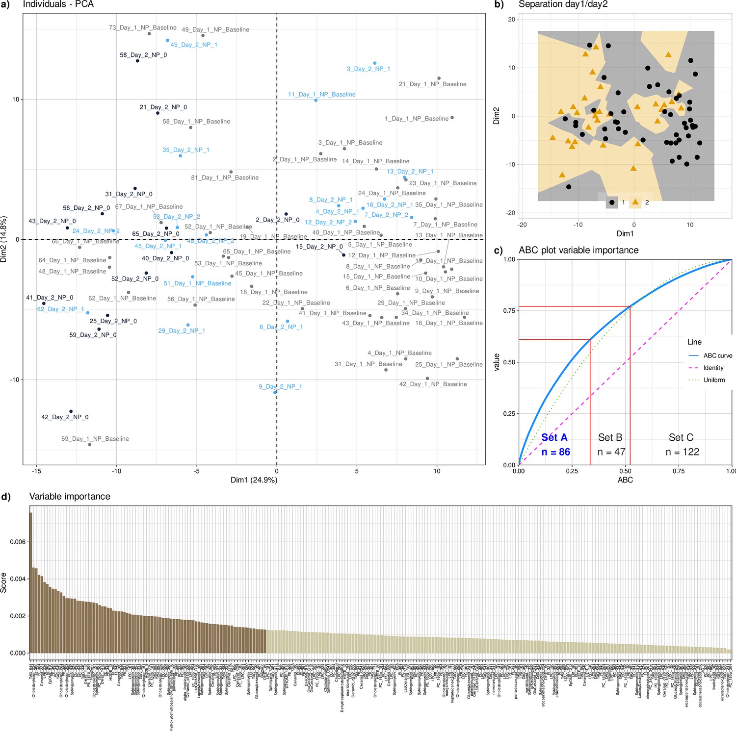
Results of a projection of the z-standardized log-transformed lipidomics data onto a lower-dimensional space by means of PCA.
(a) Projection of data set instances consisting of samples drawn before and after the paclitaxel therapy (day 1 and day 2, respectively) from patients who on day 2 were positive or negative for clinical symptoms of neuropathy. The dots indicate the positions of single data set instances on the two-dimensional plane between PC1 and PC2. They are labeled as patient number, day of sampling (1 or 2) and neuropathy (0=negative, 1=positive). (b) PCA projection, with data points are represented by their prior class membership (Day 1 and day 2). The projection plane (dimension 2 versus dimension 1) consists of Voronoi cells around each data point, colored according to the prior class membership of the respective data point. (c) ABC analysis plot (blue line) showing the cumulative distribution function of the variables contribution to the PCA projection, along with the identity distribution, xi = constant (magenta line), that is each variable has the same contribution, and the uniform distribution, that is each variable had the same chance to contribute (for further details about cABC analysis, see Gornstein and Schwarz, 2014). The red lines indicate the borders between CABC subsets ‘A’, ‘B’ and ‘C’. (d) Contribution of each lipid marker variable to the principal components normalized for the contribution of each PC in explaining the total variance. The darker brown bars indicate the mediators that were placed in category ‘A’ by a cABC analysis of variable contributions.
Figure 3
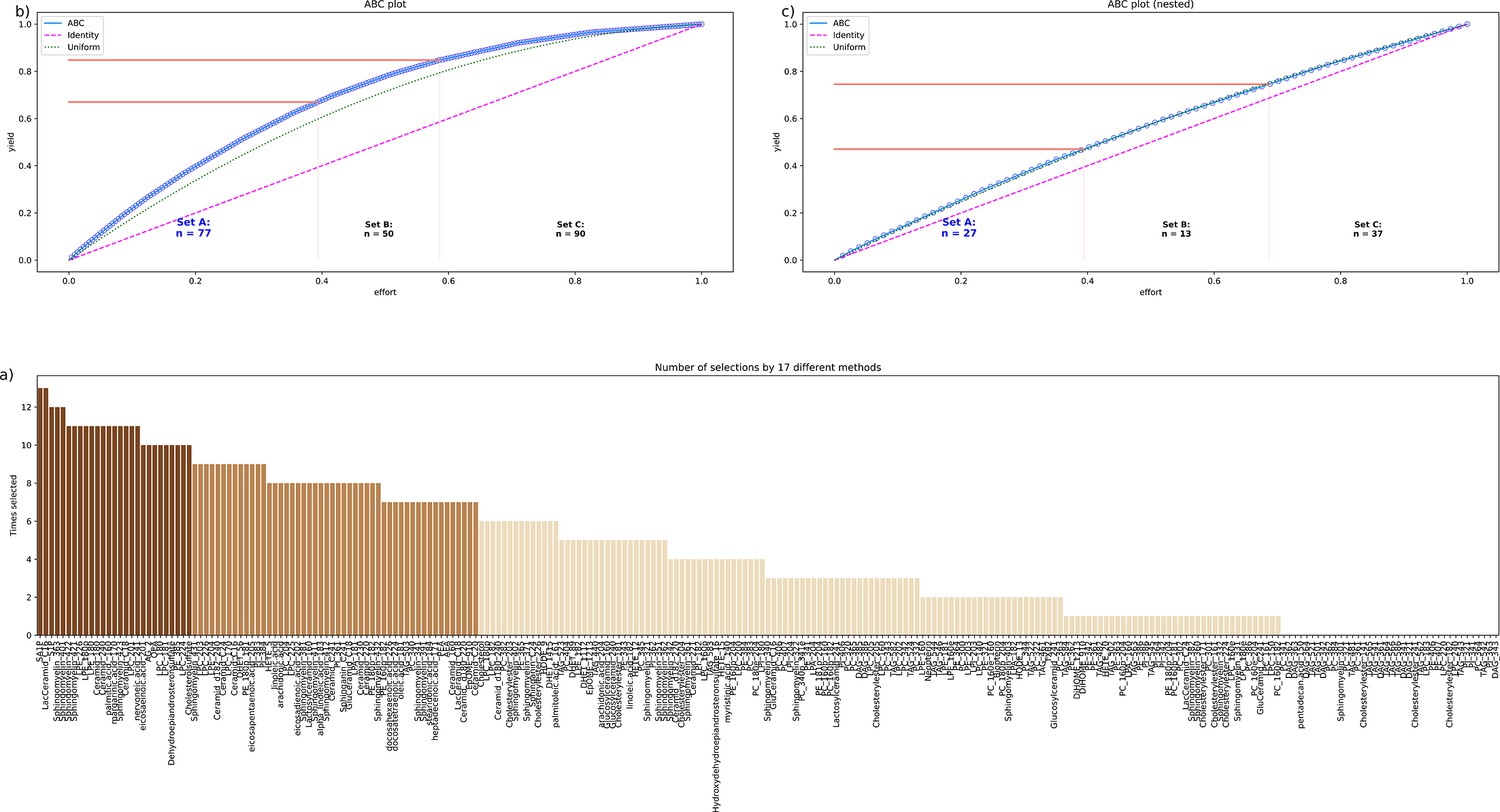
Identification of the lipid mediators that were most informative in assigning a sample to the pre- or post-therapy time point.
Feature selection by 13 different methods. (a) Bar plot of the sum score of the number of selections for each lipid marker across the 13 methods. The colors of the bars correspond to the assignments of the lipid marker to category ‘A’ in a first cABC analysis (medium brown bars) and again to category ‘A’ in a second cABC analysis performed as a nested cABC analysis (dark brown bars). Light brown bars indicate that the marker was selected by too few methods to be considered further. (b) ABC plot (blue line) showing the cumulative distribution function of the sums of selections of each marker. The red lines show the boundaries between the CABC subsets ‘A’, ‘B’, and ‘C’. Category ‘A’ with d=77 lipid mediators is considered to include the most relevant variables for sample time discrimination. (c) ABC plot of a nested cABC analysis performed on the d=77 mediators placed in category ‘A’ by a first cABC analysis. The figure was created using Python version 3.8.12 for Linux (https://www.python.org) with the seaborn statistical data visualization package (https://seaborn.pydata.org, Waskom, 2021) and our Python package ‘ABCanalysis’ (https://pypi.org/project/cABCanalysis/).
Figure 4 with 1 supplement
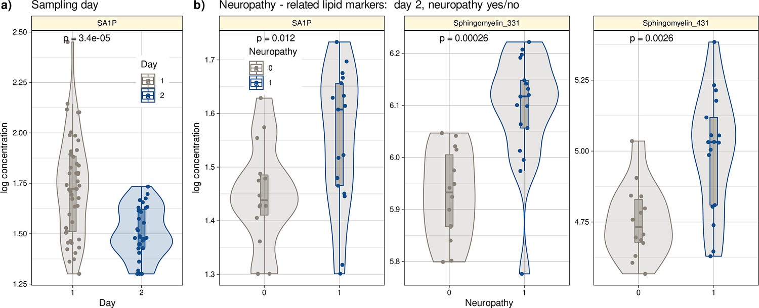
Log10-transformed concentrations of lipid mediators shown to be informative for assigning a post-therapy sample to a patient with neuropathy or a patient without neuropathy.
Individual data points are presented as dots on violin plots showing the probability density distribution of the variables, overlaid with box plots where the boxes were constructed using the minimum, quartiles, median (solid line inside the box) and maximum of these values. The whiskers add 1.5 times the interquartile range (IQR) to the 75th percentile or subtract 1.5 times the IQR from the 25th percentile. (a) Concentrations of SA1P (top hit for sample 1 versus sample 2 segregation) are presented separately for the first and second samples. (b) Concentrations of the top lipid mediators for neuropathy versus no neuropathy in the second sample presented separately for neuropathy-positive and -negative samples. The results of the group comparison statistics (Kruskal-Wallis tests Kruskal and Wallis, 1952) are given at the top of the graphs. The figure has been created using the R software package (version 4.1.2 for Linux; http://CRAN.R-project.org/, R Development Core Team, 2008) and the R library ‘ggplot2’ (https://cran.r-project.org/package=ggplot2, Wickham, 2009).
Figure 4—figure supplement 1
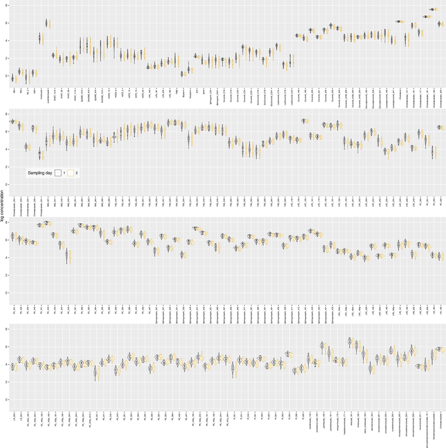
Plasma lipids from the patient cohort.
Log10-transformed concentrations of the analyzed lipid mediators presented as violin plots showing the probability density distribution of the variables. The single data points are shown as dots on overlaid on the violin plots. The presentation of the data has been arbitrarily split into two panels to enhance visibility. Sampling day 1 represents the timepoint before starting chemotherapy. Sampling day 2 represents the timepoint after 12 cycles of paclitaxel chemotherapy. The figure has been created using the R software package (version 4.1.2 for Linux; http://CRAN.R-project.org/ 1) and the R library ‘ggplot2’ (https://cran.r-project.org/package=ggplot2 2).
Figure 5 with 1 supplement
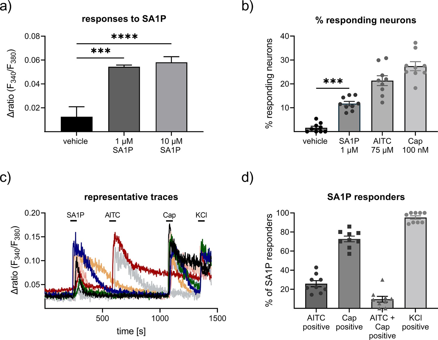
Effects of sphinganine-1-phosphate (SA1P) on primary sensory neurons.
(a) Neurons were stimulated with SA1P (1 or 10 µM, 1 min or vehicle (0.7% methanol (v/v)). (b) Percentage of responding neurons to vehicle 0.7% methanol (v/v), 1 min), SA1P (1 µM, 1 min), AITC (allyl isothioncyanate, 75 µM, 30 s), or capsaicin (Cap, 200 nM, 20 s). (c) Representative traces of SA1P-responding neurons and their response to AITC, capsaicin and KCl. (d) Percentage of SA1P-responding neurons responding to AITC, capsaicin (Cap), AITC and capsaicin and KCl. Data are shown as mean ± SEM from at least six measurements per condition with at least 40 neurons per measurement, * p<0.05, ** p<0.01, *** p<0.01, One-way ANOVA.
Figure 5—figure supplement 1
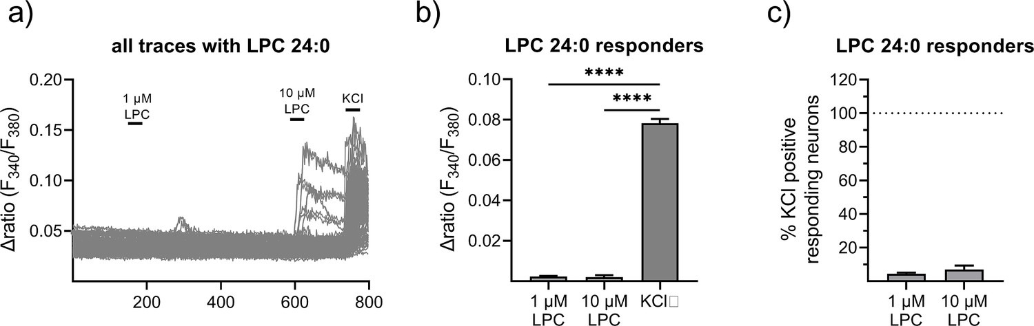
Effects of lysophosphatidylcholine 24:0 (LPC 24:0) on primary sensory neurons.
(a) Neurons were stimulated with LPC 24:0 (1 or 10 µM, 1 min) and depolarized with KCl (50 mM, 1 min) at the end of each experiment. (b) Statistical analysis of the amplitude of LPC 24:0-mediated calcium transients (1 µM, 1 min). (c) Statistical analysis of the number of LPC 24:0-responding neurons (as % of KCl-positives). Data represents mean ± SEM from at least five measurements per condition with at least 25 neurons per measurement, *** p<0.01, Student’s t-test with Welch’s correction.
Figure 6
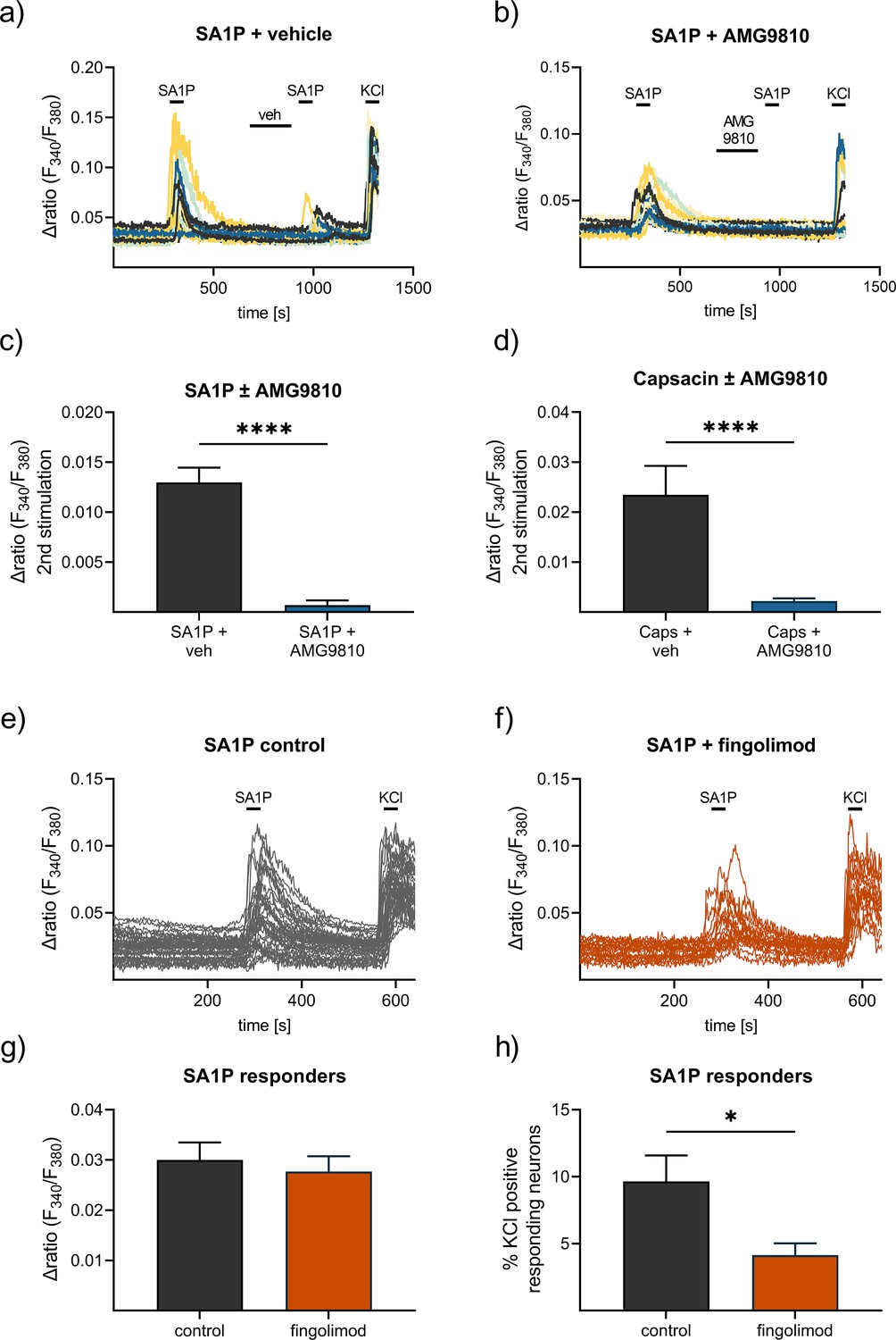
Contribution of TRPV1 and S1P receptors to SA1P-mediated calcium-influx in sensory neurons.
Sensory neurons were stimulated with SA1P twice (1 µM, 1 min) and either (a) vehicle (DMSO 0.003% (v/v), 2 min) or (b) the TRPV1 antagonist AMG9810 (1 µM, 2 min) prior to the second SA1P stimulus. Cells were depolarized with KCl (50 mM, 1 min) at the end of each experiment. (c) Statistical analysis of the amplitude of SA1P-mediated calcium transients in sensory neurons treated with either vehicle or AMG9810 (blue). (d) Statistical analysis of the amplitude of capsaicin-mediated calcium transients (Caps, 100 nM, 20 s) in sensory neurons treated with either vehicle or AMG9810 (blue). (e, f) Sensory neurons were stimulated with SA1P after preincubation with the S1P1 receptor modulator fingolimod (1 µM, 1 hr) or control. (g) Statistical analysis of the amplitude of SA1P-mediated calcium transients (1 µM, 1 min) in sensory neurons treated with either vehicle or fingolimod (1 µM, 1 hr, orange). (h) Statistical analysis of the number of SA1P-responding neurons (as % of KCl-positives) after treatment with either vehicle or fingolimod (1 µM, 1 hr, orange). Data represents mean ± SEM from at least five measurements per condition with at least 25 neurons per measurement, * p<0.05, ** p<0.01, *** p<0.01, Student’s t-test with Welch’s correction.
Figure 7 with 1 supplement
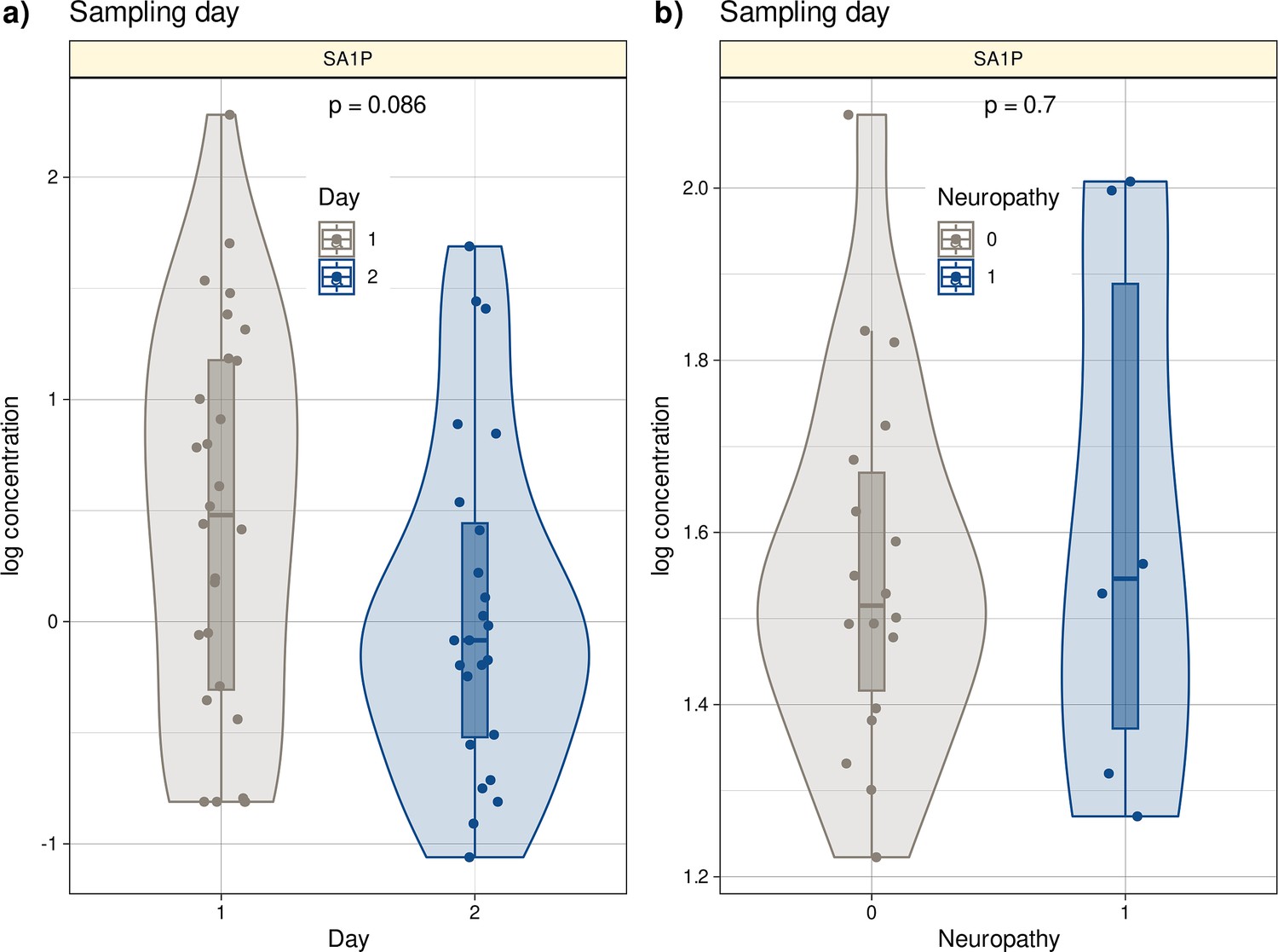
Log10-transformed concentrations of SA1P in the second patient cohort.
Individual data points are presented as dots on violin plots showing the probability density distribution of the variables, overlaid with box plots where the boxes were constructed using the minimum, quartiles, median (solid line inside the box) and maximum of these values. The whiskers add 1.5 times the interquartile range (IQR) to the 75th percentile or subtract 1.5 times the IQR from the 25th percentile. (a) Concentrations of SA1P (top hit for sample 1 versus sample 2 segregation) are presented separately for the first and second samples. (b) Concentrations of S1AP in the second sample are shown separately for neuropathy-positive and -negative samples. Day 1 represents the timepoint before starting chemotherapy. Day 2 represents the timepoint after 12 cycles of paclitaxel chemotherapy. The results of the t-test group comparison statistics are given at the top of the graphs. The figure has been created using the R software package (version 4.1.2 for Linux; http://CRAN.R-project.org/, R Development Core Team, 2008) and the R library ‘ggplot2’ (https://cran.r-project.org/package=ggplot2, Wickham, 2009).
Figure 7—figure supplement 1
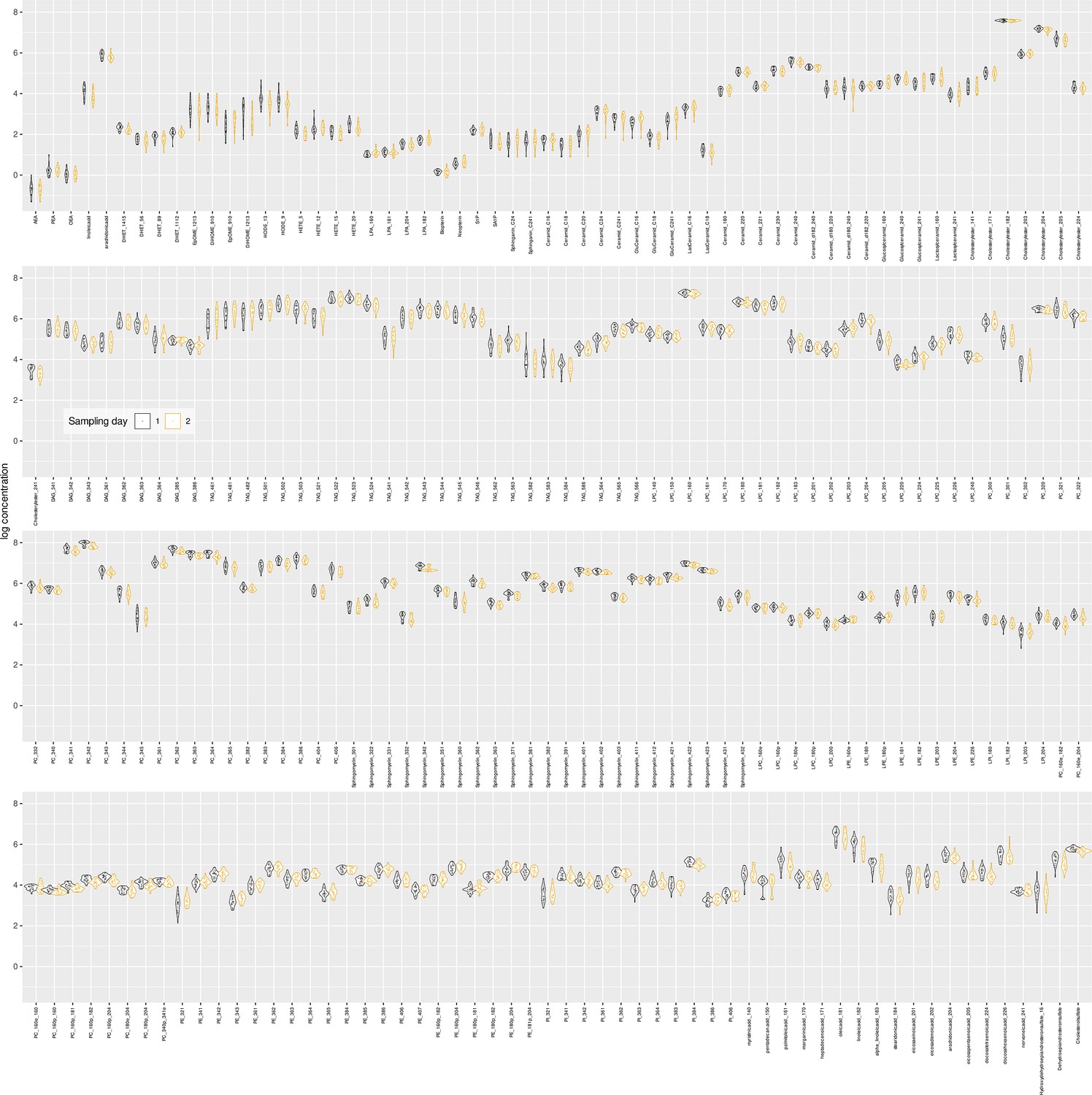
Plasma lipids from the independent second patient cohort.
Log10-transformed concentrations of the analyzed lipid mediators presented as violin plots showing the probability density distribution of the variables. The single data points are shown as dots on overlaid on the violin plots. The presentation of the data has been arbitrarily split into two panels to enhance visibility. Sampling day 1 represents the timepoint before starting chemotherapy. Sampling day 2 represents the timepoint after six cycles of paclitaxel chemotherapy. The figure has been created using the R software package (version 4.1.2 for Linux; http://CRAN.R-project.org/ 1) and the R library ‘ggplot2’ (https://cran.r-project.org/package=ggplot2 2).
Figure 8
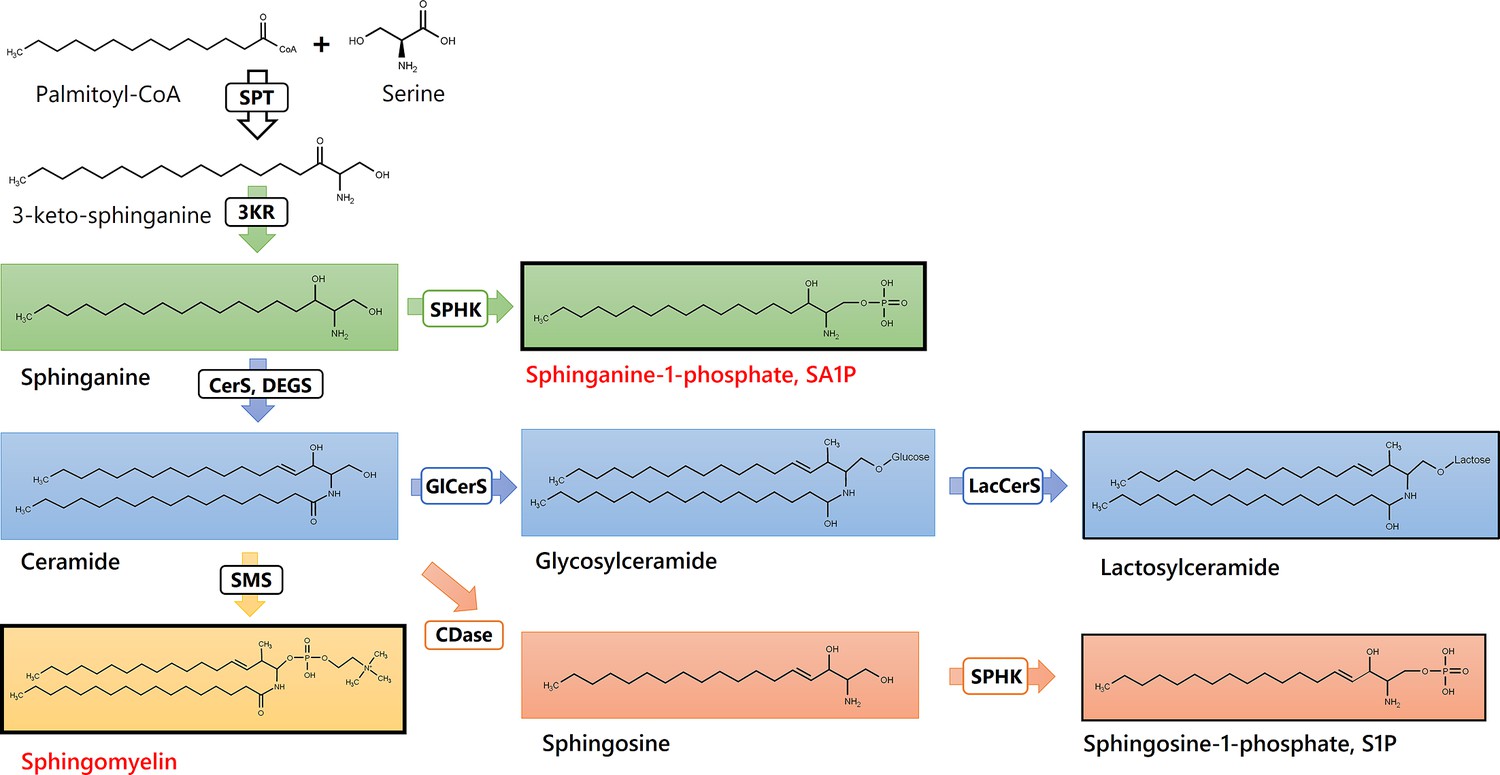
Sphingolipids and Ceramides (SPT: Serine palmitoyl-transferase; 3KR: 3-ketosphinganine reductase; SPHK: Sphingosine kinase; CerS: Ceramide synthase; DEGS: Dihydroceramide desaturase, GlCerS: Glucosylceramide synthase; LacCerS: Lactosylceramide synthase; SMS: Sphingomyelin synthase; CDase: Ceramidase).
Structures were drawn with ChemDraw 20.
Tables
Table 1
Internal validation of the sets of lipid mediators resulting from the feature selection analysis.
The different classifiers (linear support vector machine, SVM, random forests, and logistic regression) were trained with subsets of the training data set with all variables d=255 lipid mediators as ’full’ feature set and with the d=77 or d=27 lipid mediators that had resulted from the recursive cABC analysis applied on the sum score of selections by 17 different feature selection methods as ’reduced’ or ’sparse’ feature sets, respectively. The trained classifiers were applied to a validation sample comprising 20% of the data that had been removed in a class-proportional manner from the dataset at the beginning of feature selection and had not been touched until used in the classifier validation task presented in this table. In addition, the validation task was repeated with training the classifiers with permuted lipid mediators to observe possible overfitting. Shown are the medians and nonparametric 95% confidence intervals (2.5th to 97.5th percentiles) from 5x20 nested cross-validation runs.
| Classifier | Performance measure | Feature set | |||
|---|---|---|---|---|---|
| Full | Reduced | Reduced permuted | Sparse | ||
| Number of lipid mediators | 255 | 77 | 77 | 27 | |
| SVM | Balanced accuracy | 0.7 (0.48–0.92) | 0.78 (0.61–1) | 0.48 (0.23–0.76) | 0.75 (0.54–0.91) |
| Random forests | 0.7 (0.56–0.83) | 0.75 (0.58–0.85) | 0.46 (0.24–0.75) | 0.74 (0.55–0.88) | |
| Logistic regression | 0.7 (0.52–0.85) | 0.77 (0.58–0.92) | 0.48 (0.29–0.7) | 0.7 (0.49–0.89) | |
| SVM | roc-auc | 0.88 (0.67–1) | 0.95 (0.85–1) | 0.48 (0.16–0.77) | 0.9 (0.81–0.99) |
| Random forests | 0.86 (0.76–0.95) | 0.88 (0.81–0.98) | 0.48 (0.21–0.81) | 0.9 (0.8–1) | |
| Logistic regression | 0.81 (0.64–1) | 0.88 (0.75–1) | 0.46 (0.16–0.79) | 0.86 (0.69–0.98) |
Table 2
Lists of lipid mediators that were most informative in assigning a sample (i) to the first or second sampling time point or (ii) a sample from the second time point to a patient with or without neuropathy.
Abbreviations: SA1P: sphinganine-1-phosphate, S1P: sphingosine-1-phosphate, LPE: lysophosphatidylethanolamine, LPC: lysophosphatidylcholine, 2-AG: 2-arachidonoylglycerol, OEA. Oleoylethanolamide.
| Sample 1 versus sample 2 | ||||
|---|---|---|---|---|
| SA1P | Sphingomyelin 42:1 | Palmitic acid 16:0 | Eicosaeinoic acid 20:1 | PE 38:5 |
| LacCeramid C16 | LPE 22:6 | Margaritic acid 17:0 | 2-AG | LPC 22:4 |
| S1P | LPE 18:0 p | Sphingomyelin 42:3 | OEA | Cholesterolsulfate |
| Sphingomyelin 36:3 | LPE 18:0 | LPC 18:0 | Sphingomyelin 40:1 | |
| Ceramide 18:0 | LPC 20:1 | LPC 18:1 | Sphingomyelin 42:2 | |
| Ceramide 24:0 | Nervoneic acid 24:1 | Dehydroepiandrosterone sulfate | ||
| Sample 2: neuropathy versus no neuropathy | ||||
| SA1P | Sphingomyelin 33:1 | Sphingomyelin 43:1 | ||
Table 3
External validation of the classifiers in an independent patient cohort.
The different classifiers (linear support vector machine, SVM, random forests, and logistic regression) were trained with subsets of the training data set from the analysis cohort using the ‘sparse’ feature set. The trained classifiers were then applied to an independent second patient cohort. In addition, the validation task was repeated with permuted information from lipid mediators to observe possible overfitting. Shown are the medians and nonparametric 95% confidence intervals (2.5th to 97.5th percentiles) from 5x20 nested cross-validation runs.
| Classifier | Performance measure | ||
|---|---|---|---|
| Sparse | Sparse permuted | ||
| Number of lipid mediators | 27 | 27 | |
| SVM | Balanced accuracy | 0.6 (0.52–0.68) | 0.5 (0.49–0.51) |
| Random forests | 0.62 (0.5–0.68) | 0.52 (0.37–0.65) | |
| Logistic regression | 0.62 (0.54–0.74) | 0.51 (0.31–0.69) | |
| SVM | roc-auc | 0.65 (0.54–0.73) | 0.51 (0.19–0.72) |
| Random forests | 0.66 (0.55–0.75) | 0.52 (0.24–0.76) | |
| Logistic regression | 0.69 (0.6–0.78) | 0.49 (0.25–0.78) |
Additional files
-
Supplementary file 1
Table of patient characteristics of the 31 patients that gave blood samples before and after chemotherapy from the patient cohort.
- https://cdn.elifesciences.org/articles/91941/elife-91941-supp1-v1.xlsx
-
Supplementary file 2
Complete list of lipid mediators included in the analyses, separated by group of lipid and detection method.
- https://cdn.elifesciences.org/articles/91941/elife-91941-supp2-v1.xlsx
-
Supplementary file 3
Table of patient characteristics of the 28 patients from the second cohort that gave blood samples before and after the sixth cycle of chemotherapy.ld like to thank Drs Tabea Ost.
- https://cdn.elifesciences.org/articles/91941/elife-91941-supp3-v1.xlsx
-
MDAR checklist
- https://cdn.elifesciences.org/articles/91941/elife-91941-mdarchecklist1-v1.pdf
Download links
A two-part list of links to download the article, or parts of the article, in various formats.
Downloads (link to download the article as PDF)
Open citations (links to open the citations from this article in various online reference manager services)
Cite this article (links to download the citations from this article in formats compatible with various reference manager tools)
Machine learning and biological validation identify sphingolipids as potential mediators of paclitaxel-induced neuropathy in cancer patients
eLife 13:RP91941.
https://doi.org/10.7554/eLife.91941.3


