Neuro-evolutionary evidence for a universal fractal primate brain shape
- CNNP Lab (https://www.cnnp-lab.com), School of Computing, Newcastle University, United Kingdom
- Faculty of Medical Sciences, Newcastle University, United Kingdom
- UCL Institute of Neurology, Queen Square, United Kingdom
- School of Psychology, University of Nottingham, United Kingdom
- Department of Neurosurgery, University of Iowa, United States
- metaBIO Lab, Instituto de Física, Universidade Federal do Rio de Janeiro (UFRJ), Brazil
Figures
Figure 1
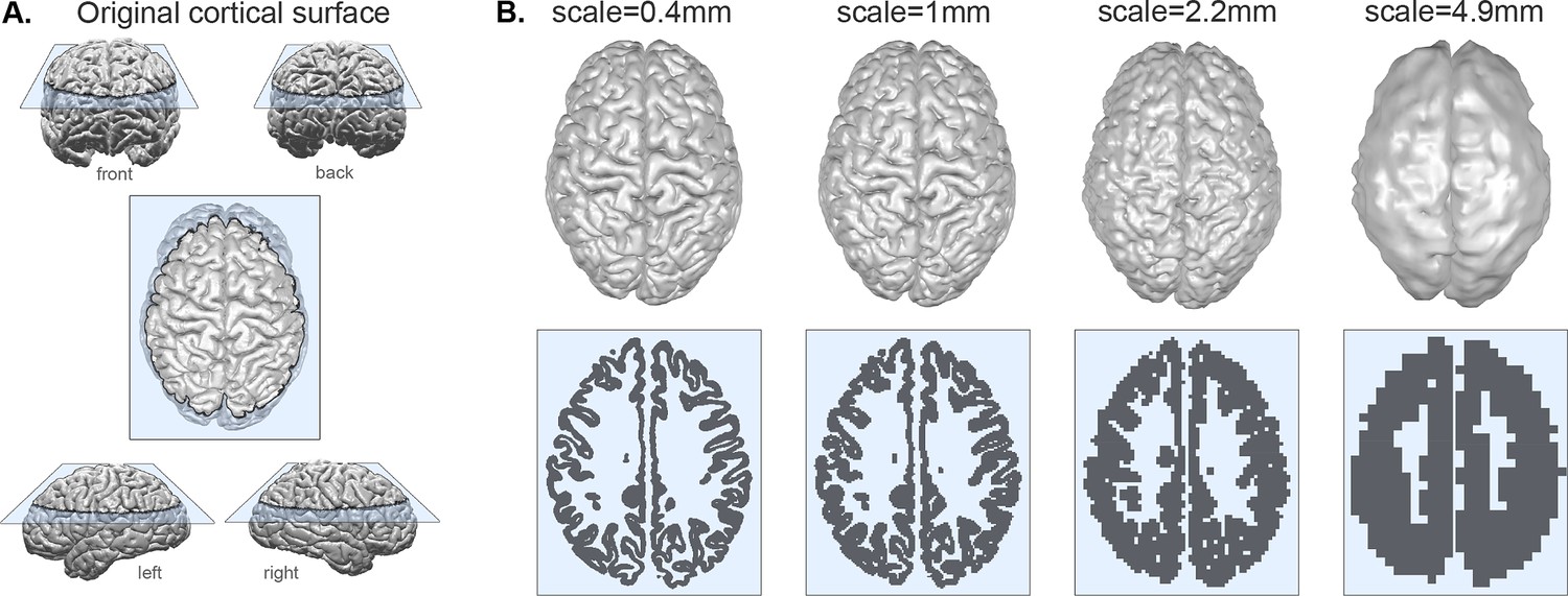
Coarse-graining a cortex at different scales.
(A) Example of original pial surface from a healthy human viewed from varying angles. (B) Same example cortical surface from A, coarse-grained to different spatial scales. Top row shows the resulting pial surfaces (with a small amount of smoothing applied for visualisation purposes here). Bottom row shows the corresponding voxelisation at each scale through the slice indicated by the blue plane in panel A. Note that the actual size of the brains for analysis is rescaled (see Methods and Figure 2); we display all brains scaled at an equal size here for the ease of visualisation of the method.
Figure 2
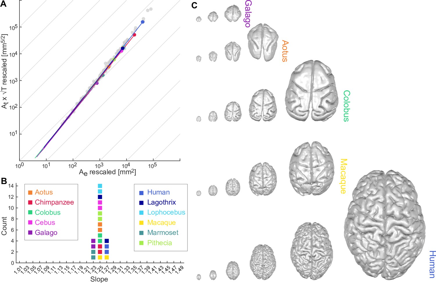
Universal scaling law for 11 coarse-grained primate brains.
(A) Coarse-grained primate brains are shown in terms of their relationship between log10 () vs. log10 (). Each solid line indicates a cortical hemisphere from a primate species. Thin grey lines indicate a slope of 1 for reference. Filled circles mark the data points of the original cortical surfaces. Grey data points are plotted for reference and show the comparative neuroanatomy dataset across a range of mammalian brains (Mota and Herculano-Houzel, 2015). (B) Slopes () of the regression of data points in A for each species. For each species, two data points are shown, one per hemisphere. Colour-code for each species is maintained throughout the whole figure. (C) Rescaled brain surfaces visualised for five example species at different levels of coarse-graining.
Figure 3
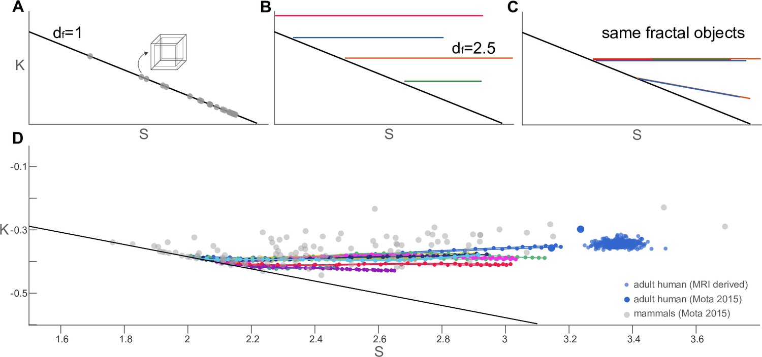
Trajectories of coarse-grained primate cortices and other mammalian and human brains in plane.
(A) Straight trajectories indicate self-similarity (described by a scaling law). In particular, the black line here indicates objects with for all scales, such as the box of finite thickness with a fractal dimension (grey data points). This line is reproduced in all subpanels for reference. (B) Morphological trajectories of multiple hypothetical fractal objects are shown which. A flat trajectory (constant ) corresponds to in this space. However, these objects are clearly different fractals with different values of . (C) Hypothetical objects with overlapping straight morphological trajectories indicate multiple realisations of the same fractal object. Flat trajectories (constant ) correspond to . The two hypothetical objects with a decreasing correspond to (D) Projecting our actual data into the normalised plane showing the coarse-grained primate brains (same as in Figure 2) as data point connected with solid lines (colour-code same as Figure 2). Different mammalian brains are shown as grey scatter points, and adult human data points are blue.
Figure 4
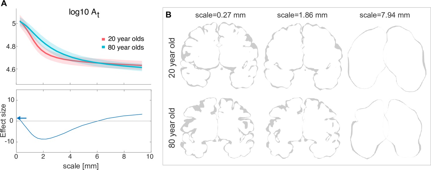
Human ageing shows differential effects depending on spatial scale.
(A) Top: is shown for a group of 20-year-olds (red, n=27) and a group of 80-year-olds (blue, n=86). Mean and standard deviation are shown as the solid line and the shaded area, respectively. Bottom: Effect size (measured as rank sum z-values) between the older and younger groups at each scale. Positive effect indicates a larger value for the younger group. Blue arrows indicate the effect size at the ‘native scale’ i.e., using the original free surfer grey and white matter meshes. (B) Coronal slices of the pial surface of an example 20-year-old subject and an 80-year-old subject at different scales (columns).
Appendix 2—figure 1
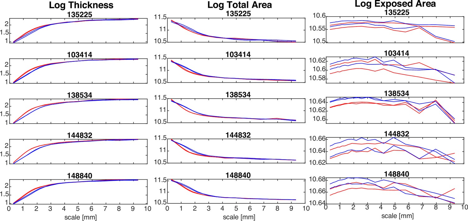
Effect of using different original image resolutions in five examples Human Connectome Project (HCP) subjects.
In all plots, red lines indicate an original image resolution of 0.7 mm isotropic, whereas blue line indicate an original image resolution of 1 mm isotropic. Both hemispheres are shown for each subject.
Appendix 3—figure 1
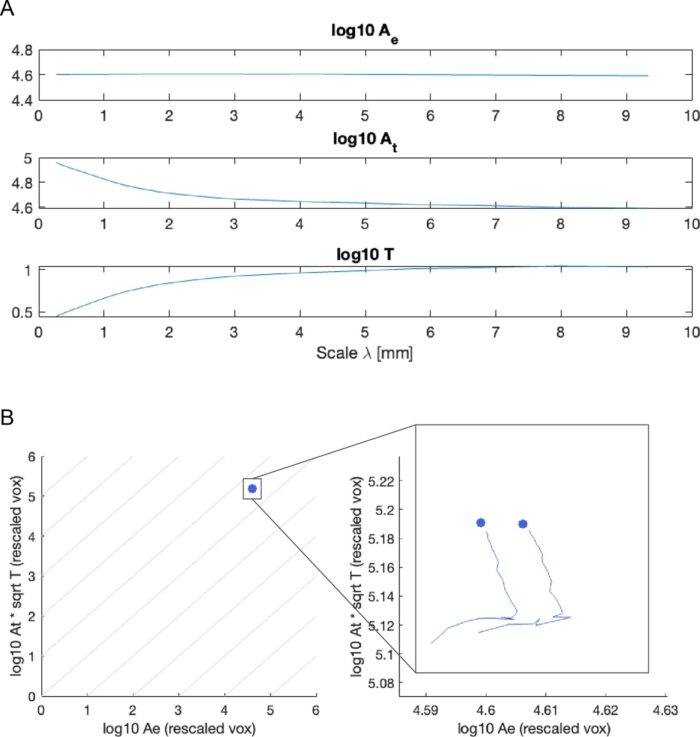
Unscaled quantities cannot be used to verify scaling law.
(A) The exposed surface area barely changes across scales, and only changes minimally. (B) Plotted in the scaling law plane (as Figure 2) the data points barely have any variance, and overlap each other substantially. Even after zooming in, the trace for the coarse-graining procedure (solid line) is virtually a vertical line (with a small artifactual ‘tail’ coming from very large voxel sizes).
Appendix 3—figure 2
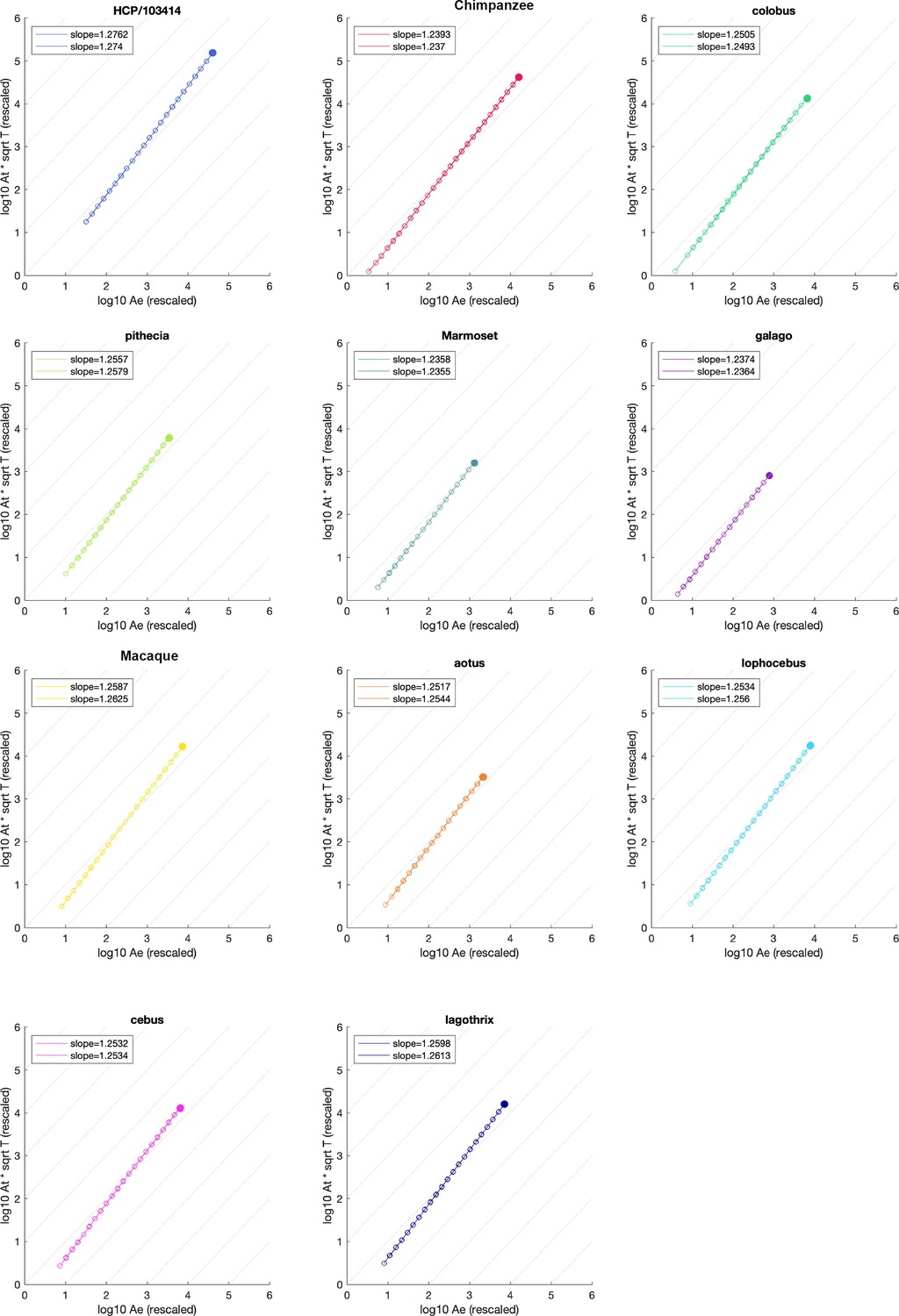
Detailed scaling plots for each species.
Filled circle is the original mesh, empty circle are data points from the coarse-graining algorithm. Empty circles are connected by a line for visualisation. Two hemispheres are analysed and separated for each species, although data points overlap substantially in plot. Slope estimates are given at top left corner in each plot.
Appendix 5—figure 1
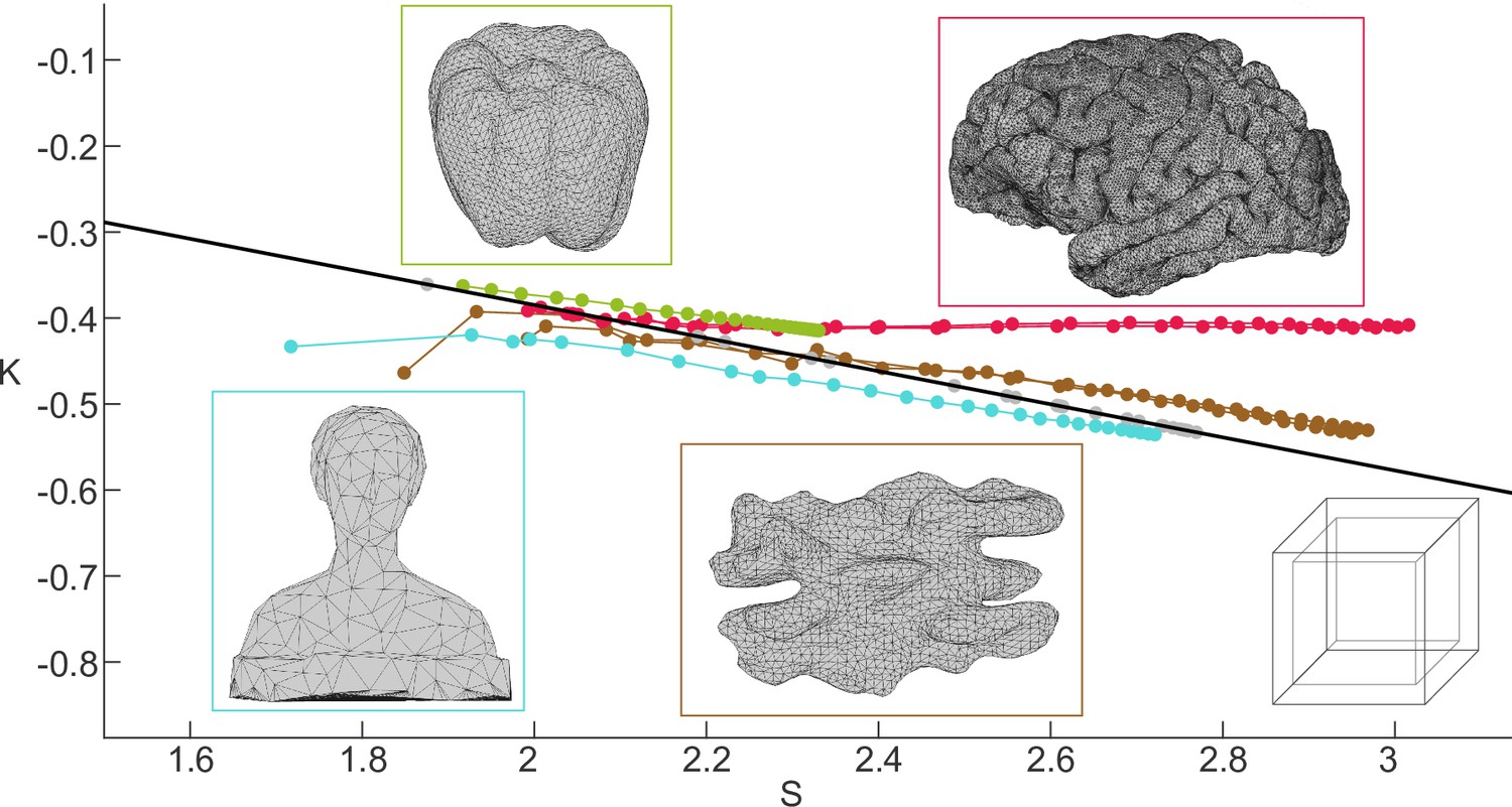
Scaling behaviour of various objects in space.
Thick black line indicates and a gyrification index. Points above and below the line have, respectively, and . Colour-coded boxes show the surface of the objects we analysed. For simplicity we show the outer ‘pial’ surface of each object. In the case of the box, we indicated both outer and inner surfaces. Green data points correspond to the bell pepper, red to the human brain, cyan to the ‘Laurana’ bust, brown to the walnut, and grey to the box of finite thickness.
Appendix 6—figure 1
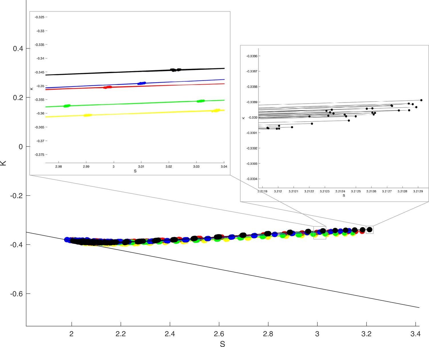
Randomising grid for coarse-graining yields very consistent results within individuals in space.
Thick black line indicates and a gyrification index . Each colour in the plot indicates a different human individual (Human Connectome Project, HCP 103414 - yellow, 135225 - red, 138534 - green, 144832 - blue, 148840 - black, respectively). 30 jittered grid outputs are shown for each individual, lines connect datapoints of the same jittered version. Zoomed in panels show that the jittered outputs have far less variation within than between individuals.
Appendix 7—figure 1
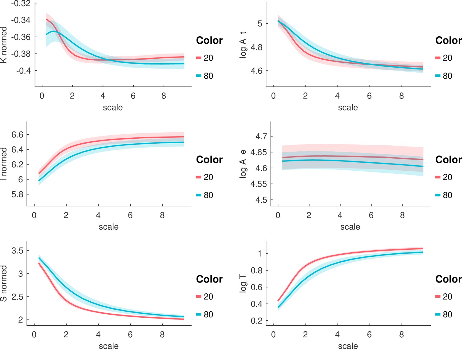
All morphological variables across scales in the 20 y.o. and 80 y.o. cohort.
Each panel shows a morphological metric, and data is shown for a group of 20-year-olds (red, n=27) and a group of 80-year-olds (blue, n=86). Mean and standard deviation are shown as the solid line and the shaded area, respectively.
Appendix 7—figure 2

Effect size between the 20 y.o. and 80 y.o. cohort in all morphological variables.
Each panel shows a morphological metric, and data is shown for a group of 20-year-olds (red, n=27) and a group of 80-year-olds (blue, n=86). Effect size is measured as the rank sum z statistic between the two groups.
Appendix 7—figure 3
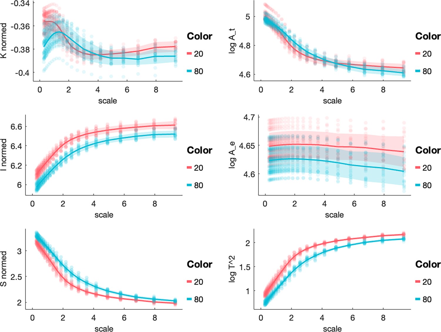
All morphological variables across scales in the 20 y.o. and 80 y.o. cohort in a separate (NKI) dataset.
Each panel shows a morphological metric, and data from an independent dataset (NKI) is shown for a group of 20-year-olds (red, n=10) and a group of 80-year-olds (blue, n=10).
Appendix 7—figure 4
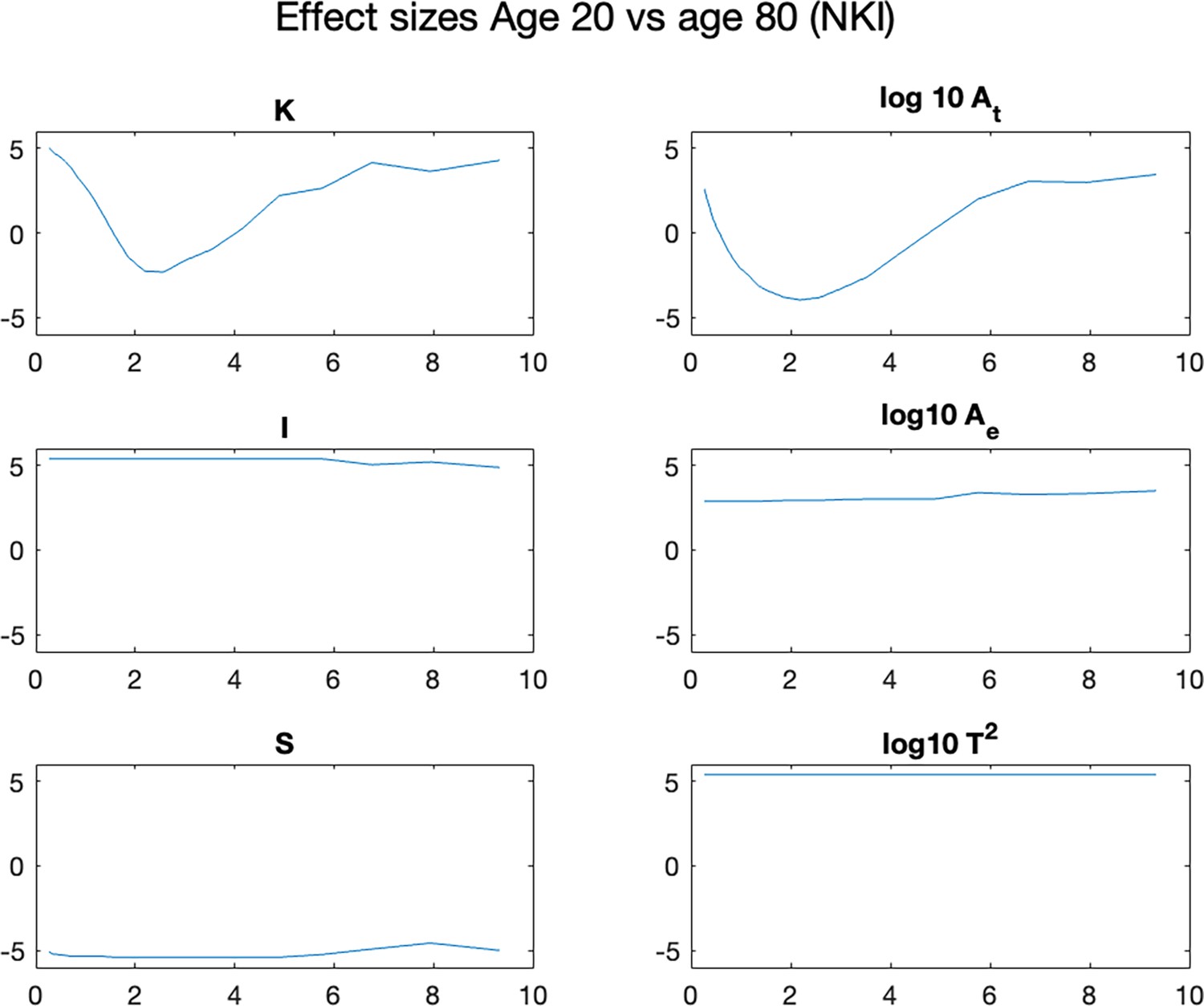
Effect size between the 20 y.o. and 80 y.o. cohort in all morphological variables in a separate (NKI) dataset.
Effect size is measured as the rank sum z statistic between the two groups. Mean and standard deviation are shown as the solid line and the shaded area, respectively.
Additional files
Download links
A two-part list of links to download the article, or parts of the article, in various formats.
Downloads (link to download the article as PDF)
Open citations (links to open the citations from this article in various online reference manager services)
Cite this article (links to download the citations from this article in formats compatible with various reference manager tools)
Neuro-evolutionary evidence for a universal fractal primate brain shape
eLife 12:RP92080.
https://doi.org/10.7554/eLife.92080.4


