A scenario for an evolutionary selection of ageing
Figures
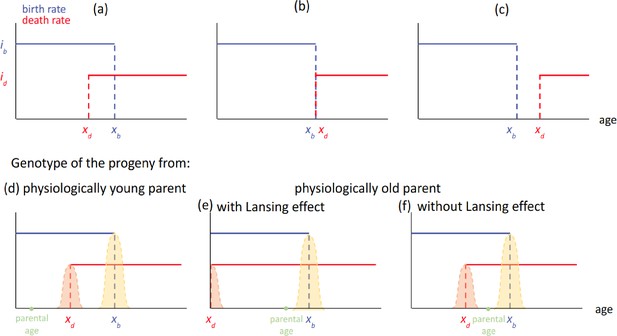
Three typical configurations of the model with ib >id and their effect on progeny’s genotypes as a function of parental age.
(upper panel) Each haploid individual is defined by a parameter xb defining its fertility span of intensity ib and a parameter xd defining the time during which it will maintain itself, with an intensity id. These parameters can be positive or null. (a) ’Too young to die’: it corresponds to configurations satisfying xd <xb. (b) ’Now useless’: it corresponds to configurations where xb = xd. (c) ‘Menopause’: it corresponds to configurations where xd >xb. (lower panel) Each individual may randomly produce a progeny during its fertility span [0; xb]. (d) In the case of physiologically young parents (a<xd), the progeny’s genotype is that of its parent ∓ a Gaussian kernel of mutation centered on the parental gene. In the case of the reproduction event occurring after xd, for configuration (a) above, two cases are observed, (e) if the organism carries a Lansing effect ability, the xd of its progeny will be strongly decreased. (f) In the absence of the Lansing effect, the default rule applies.

The bd model shows a convergence of xb - xd towards a positive value.
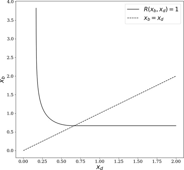
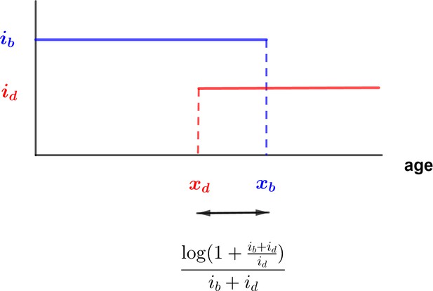
Dynamics of the individual-based model shows a convergence of xb - xd towards a positive constant value in the absence of the Lansing effect. (a) The generalized b-d model shows a convergence of (xb - xd) for any ib and id towards a positive value given by (b) (Annexe 4.3, Figure 2). (c) Simulation of 1000 individuals with initial trait (xb=1.2, xd=1.6) of intensities ib=id=1, a competition c=0.0009 and a mutation kernel (P=0.1, σ=0.05) show that the two parameters co-evolvetowards xb - xd ≅ 0.55 that is log(3)/2. (d) Landscape of solutions (xb - xd) as a function of ib and id (colors separate ranges of 50 units on the z-axis).
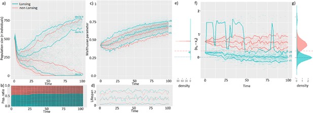
The Lansing effect maximizes populational survival by increasing its evolvability.
100 independent simulations were run with a competition intensity of 9.10–4 and a mutation rate p=0.1 on a mixed population made of 500 non-Lansing individuals and 500 individuals subjected to such effect. At t0, the population size exceeds the maximum load of the medium thus leading to a population decline at start. At t0, all individuals are of age 0. Here, we plotted a subset of the 100.106 plus individuals generated during the simulations. Each individual is represented by a segment between its time of birth and its time of death. In each graph, blue and red curves represent deciles 1, 5, and 9 of the distribution at any time for each population type. (a) The higher success rate of Lansing bearing populations does not seem to be associated with a significantly faster population growth but with a lower risk of collapse. (b) For cohabitating populations, the Lansing bearing population (blue) is overgrowing by only 10% the non-Lansing one (red). (c) This higher success rate is associated with a faster and broader exploration of the Malthusian parameter - surrogate for fitness - space in Lansing bearing populations (d) that is not associated with significant changes in the lifespan distribution (e) but a faster increase in genotypic variability within the [0; 10] time interval. (f) This occurs although progeny from physiologically old parents can represent up to 10% of the Lansing bearing population and leads to it reaching the theoretical optimum within the timeframe of simulation (g) with the exception of Lansing progenies. (e–g) Horizontal lines represent the theoretical limits for (xb - xd) in Lansing (blue) and non-Lansing (red) populations.

Evolution of the average Malthusian parameter value in Lansing and non-Lansing populations as a function of time.
p is the mutation rate and c is the logistic competition intensity. Individual values are plotted, the line represents the average value amongst populations. In all conditions with p > 0, the Malthusian parameter grows faster and remains slightly higher in the Lansing populations than in the non-Lansing ones.

Evolution of the Lansing and non-Lansing populations size as a function of time.
p is the mutation rate and c is the logistic competition intensity.
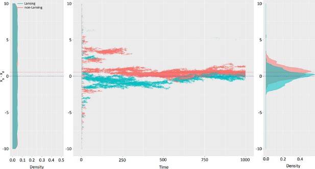
Mixed populations lead to (xb - xd) theoretical limit in a limited time and cohabitation of Lansing and non-Lansing populations.
Starting with a homogenous population of 5000 Lansing bearing and 5000 non-Lansing individuals with traits uniformly distributed from –10 to +10 (left panel), we ran 100 independent simulations on time in [0; 1000]. (center panel) Plotting the trait (xb - xd) as a function of time for one simulation shows a rapid elimination of extreme traits and branching evolution. (right panel) The final distribution of traits in each population type is centered on the theoretical convergence limit for each. Ntotal ≅ 110 millionindividuals, c=9.10–4, p=0.1.
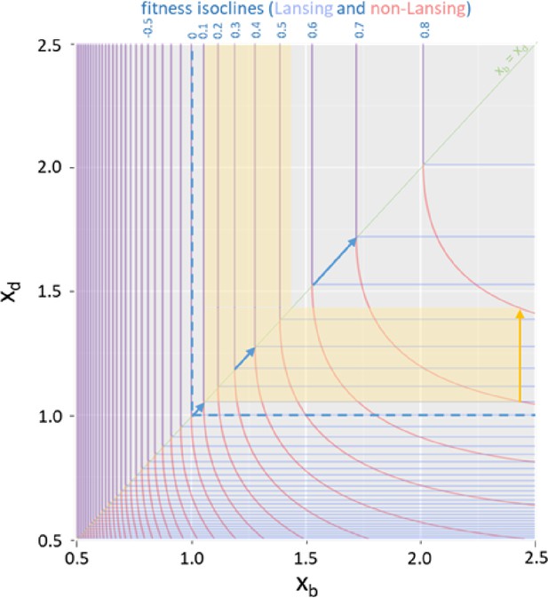
The Lansing effect is associated with an increased fitness gradient.
We were able to derive Lansing and non-Lansing Malthusian parameters from the model’s equations (see Annexe 1–2.3 and 1–5) and plot them as a function of the trait (xb, xd). The diagonal xb = xd is drawn in light green. The corresponding isoclines are overlapping above the diagonal but significantly differ below, with non-Lansing fitness (red lines) being higher than that of Lansing’s (light blue lines). In addition, the distance between two consecutive isoclines is significantly more important in the lower part of the graph for non-Lansing than Lansing bearing populations. As such, a mutation leading a non-Lansing individual’s fitness going from 0.7 to 0.8 (yellow arrow) corresponds to a Lansing individual’s fitness going from 0.1 to 0.52. Finally, Hamilton’s decreasing force of selection with age can be observed along the diagonal with a growing distance between two consecutive fitness isoclines as xb and xd continue increasing.
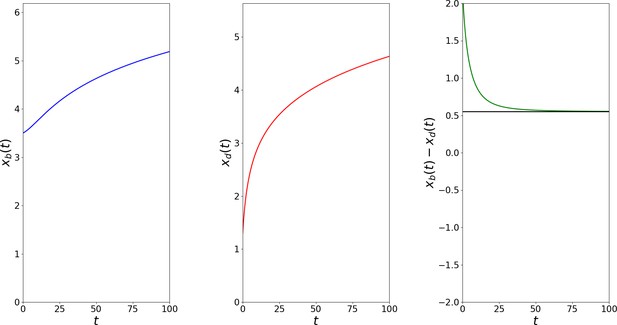
Simulation of the canonical equation with and .
(a) Dynamics of xb. (b) Dynamics of xd. (c) Dynamics of, the black curve has equation. .
Tables
Populations with Lansing effect are favorably selected under logistic competition when the mutation rate is non-zero.
p is the mutation rate and c the intensity of the logistic competition. For each couple (p, c), 100 independent simulations were run with 500 individuals per population at t0 of which traits are (1.5; 1.3) Lansing and (1.5; 0.83)non-Lansing so that their respective Malthusian parameters are equal. Each simulation corresponds to 2.105 events of birth or death. Table (a) shows the ratio of Lansing and non-Lansing populations (out of 100 simulations in each case) that did collapse by the end of the simulation. For the lowest competition, none of the populations collapsed within the timeframe of simulations (-). For an intermediate value of competition, approximately less than half of Lansing populations disappear, relative to non-Lansing ones. Table (b) shows the ratio of the number of individuals generated between Lansing and non-Lansing populations. On average, Lansing populations generate approximately twice as many individuals as non-Lansing ones. (c) On average, Lansing populations grow 20% more than the non-Lansing. Values highlighted in green are discussed further below.
| Mutation probability | |||||||||||||
|---|---|---|---|---|---|---|---|---|---|---|---|---|---|
| 0 | 0.1 | 0.5 | 1 | 0 | 0.1 | 0.5 | 1 | 0 | 0.1 | 0.5 | 1 | ||
| a) Lansing/non-Lansing collapsed population | b) Lansing/non-Lansing number of individuals | c) Lansing/total population size | |||||||||||
| Competition | 9.10–5 | - | - | - | - | 1.30 | 1.38 | 1.39 | 1.35 | 0.57 | 0.64 | 0.62 | 0.59 |
| 9.10–4 | 1.02 | 0.62 | 0.56 | 0.66 | 1.70 | 2.84 | 3.58 | 3.20 | 0.49 | 0.62 | 0.60 | 0.55 | |
| 9.10–3 | 1.00 | 1.05 | 1.13 | 1.03 | 1.05 | 1.31 | 1.56 | 1.84 | - | 0.43 | 0.44 | 0.49 | |
-
Table 1—source data 1
The magnitude of the Lansing effect does not influence the outcome of evolution.
100 independent simulations were run for each Lansing effect magnitude ranging from 0 (no Lansing effect) to 1 (progeny from parents age € [xd; xb] have xd = 0), starting with 500 Lansing (1.5; 1.3) and 500 non-Lansing (1.5; 0.83) individuals. We plot here the distribution density of xb - xd at the end of the simulation (individuals born in the time interval [990; 1000]), for Lansing populations (blue) and non-Lansing ones (red). Surprisingly, the magnitude of the Lansing effect does not seem to affect the optimal xb - xd solution value.
- https://cdn.elifesciences.org/articles/92914/elife-92914-table1-data1-v1.zip


