Intraspecific predator interference promotes biodiversity in ecosystems
- School of Physics, Sun Yat-sen University, China
- School of Mathematics, Sun Yat-sen University, China
- Department of Mechanical Engineering, Massachusetts Institute of Technology, United States
Figures
Figure 1
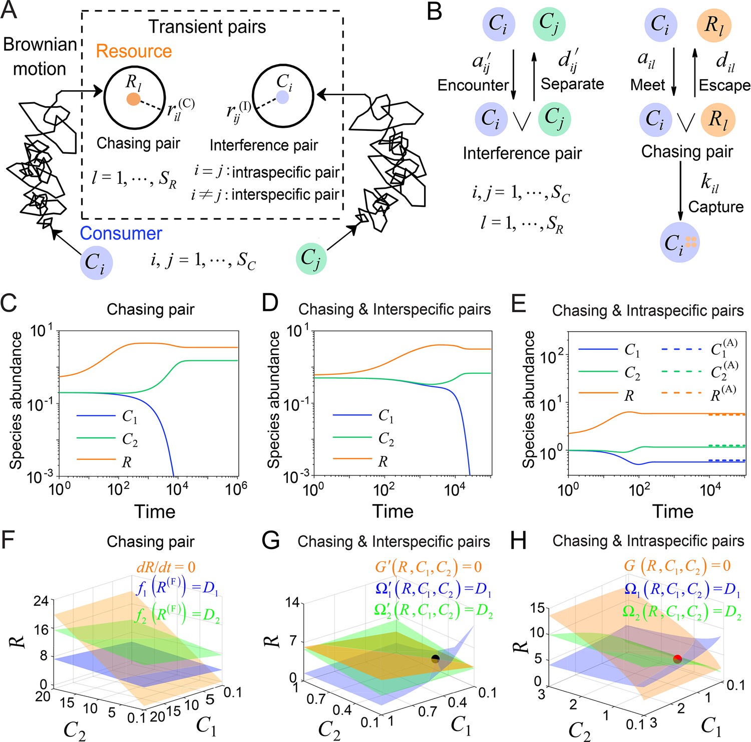
A model of pairwise encounters may naturally break CEP.
(A) A generic model of pairwise encounters involving consumer species and resource species. (B) The well-mixed model of (A). (C–E) Time courses of two consumer species competing for one resource species. (F–H) Positive solutions to the steady-state equations (see Equations S38 and S65): (orange surface), (blue surface), (green surface), that is the zero-growth isoclines. The black/red dot represents the unstable/stable fixed point, while the dotted lines in (E) are the analytical solutions of the steady-state abundances (marked with superscript ‘(A)’). See Appendix 1—tables 1 and 2 for the definitions of symbols. See Appendix 9 for simulation details.
Figure 2
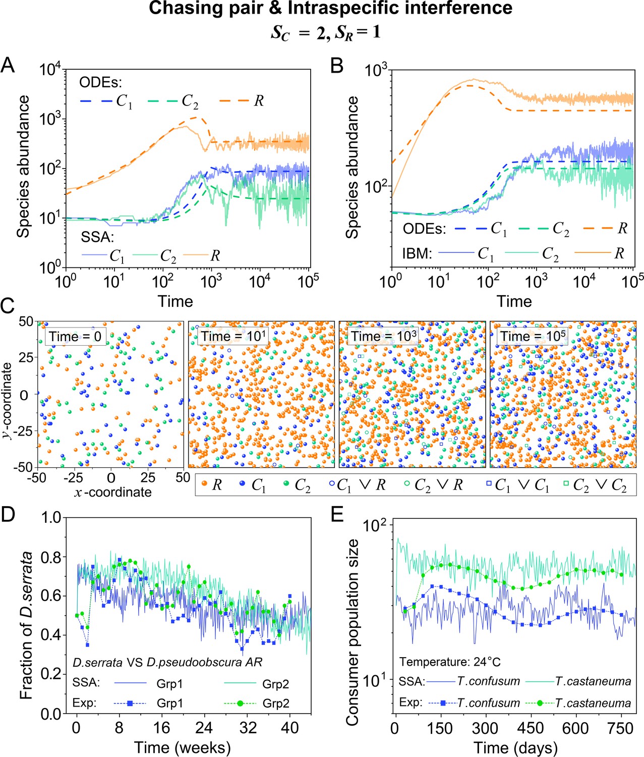
Intraspecific predator interference facilitates species coexistence regardless of stochasticity.
(A, B) Time courses of the species abundances simulated with ODEs, SSA, or IBM. (C) Snapshots of the IBM simulations. (D, E) A model of intraspecific predator interference explains two classical laboratory experiments that invalidate CEP. (D) In Ayala’s experiment, two Drosophila species coexist with one type of resources within a laboratory bottle (Ayala, 1969). (E) In Park’s experiment, two Tribolium species coexist for 2 years with one type of food (flour) within a lab (Park, 1954). See Appendix 1—figure 7C, D for the comparison between model results and experimental data using Shannon entropies.
Figure 3

Intraspecific interference enables a wide range of consumer species to coexist with only one or a handful of resource species.
(A, B) Representative time courses simulated with ODEs and SSA. (C, D) A model of intraspecific predator interference illustrates the S-shaped pattern of the species’ rank-abundance curves across different ecological communities. The solid icons represent the experimental data (marked with ‘Exp’) reported in existing studies (Fuhrman et al., 2008; Cody and Smallwood, 1996; Terborgh et al., 1990; Martínez et al., 2023; Clarke et al., 2005; De Vries, 1997; Hubbell, 2001), where the bird community data were collected longitudinally in 1982 and 2018 (Terborgh et al., 1990; Martínez et al., 2023). The ODEs and SSA results were constructed from timestamp in the time series. In the K-S test, the probabilities (p-values) that the simulation results and the corresponding experimental data come from the same distributions are: , , , , , , , , , . See Appendix 9 for simulation details and the Shannon entropies.
Appendix 1—figure 1

Estimation of the encounter rates with the mean-field approximations.
To calculate in the chasing pair, we suppose that all individuals of species stand still while a individual moves at the speed of (the relative speed). Over a time interval of , the length of zigzag trajectory of the individual is approximately , while the encounter area (marked with dashed lines) is estimated to be . Then, we can estimate the encounter rate using the encounter area and concentrations of the species (see Materials and methods for details). Similarly, we can estimate in the interference pair.
Appendix 1—figure 2
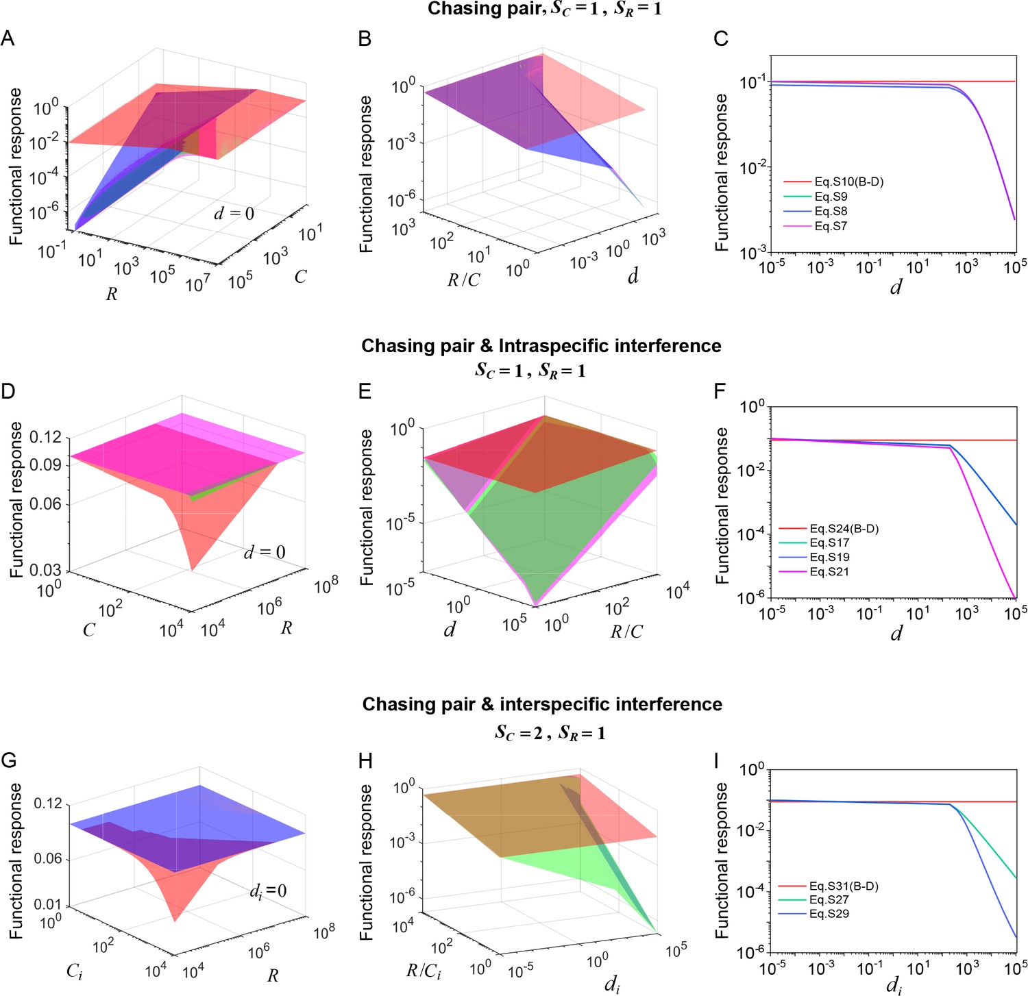
Functional response in scenarios involving different types of pairwise encounter.
(A–C) In the scenario involving only chasing pair, the red surface/line corresponds to the B-D model (calculated from Equation S10b), while the green surface/line represents the exact solutions to our mechanistic model (calculated from Equation S7b). The magenta (calculated from Equation S8b) and blue (calculated from Equation S9b) surfaces/lines represent the approximate solutions to our model (see Appendix 3.B). (D–F) In the scenario involving chasing pairs and intraspecific interference, the red surface/line corresponds to the B-D model (calculated from Equation S24b), while the green/line surface represents the exact solutions to our mechanistic model (calculated from Equation S17b). The blue surface/line (calculated from Equation S19b) and the magenta surface/line (calculated from Equation S21b) represent the quasi-rigorous and the approximate solutions to our model, respectively (see Appendix 3.C). (G–I) In the scenario involving chasing pairs and interspecific interference, the red surface/line corresponds to the B-D model (calculated from Equation S31b), while the green surface/line represents the quasi-rigorous solutions to our mechanistic model (calculated from Equation S27d). The blue surface/line (calculated from Equation S29d) represents the approximate solutions to our model (see Appendix 3.D). In (A–C): , . In (A): . In (C): , . In (D–F): , , , . In (D): . In (F): , . In (G–I): , , , . In (G): . In (I): , .
Appendix 1—figure 3
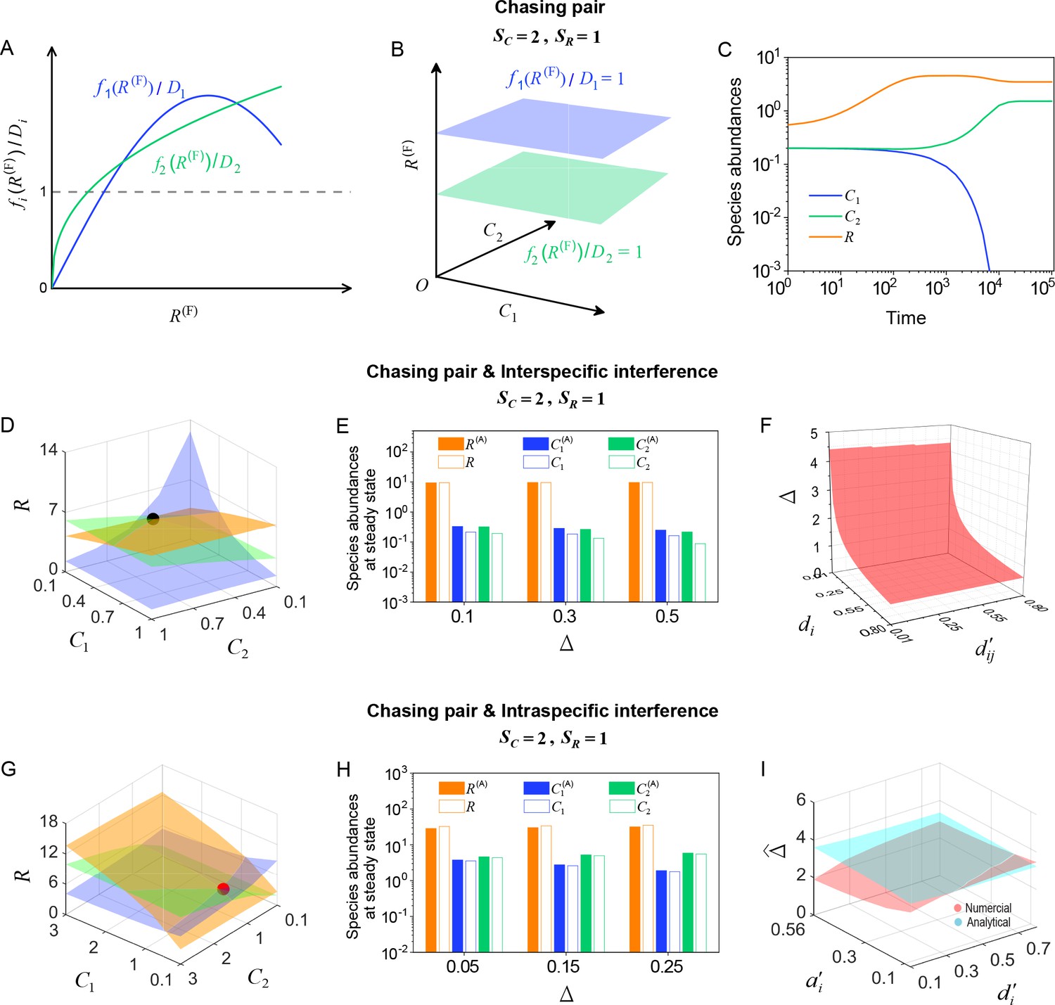
Numerical solutions in scenarios involving chasing pairs and different types of predator interference.
Here, and . is the only parameter varying with the consumer species (with ), and represents the competitive difference between the two species. (A–C) Scenario involving only chasing pairs. (A) If all consumer species coexist at steady state, then , where and . This requires that the three lines and share a common point, which is generally impossible. (B) The blue plane is parallel to the green one, and hence they do not have a common point. (C) Time courses of the species abundances in the scenario involving only chasing pairs. The two consumer species cannot coexist at steady state. (D–F) Scenario involving chasing pairs and interspecific interference. (G–I) Scenario involving chasing pairs and intraspecific interference. (D, G) Positive solutions to the steady-state equations: (orange surface), (blue surface), (green surface). The intersection point marked by black/red dots is an unstable/stable fixed point. (E, H) Comparisons between the numerical results and analytical solutions of the species abundances at fixed points. Color bars are analytical solutions while hollow bars are numerical results. The analytical solutions in (E) and (H) (marked with superscript ‘(A)’) were calculated from Equations S68 and S70 and Equation S41, Equation S43, respectively. (F) In this scenario, there is no parameter region for stable coexistence. The region below the red surface and above represents unstable fixed points. (I) Comparisons between the numerical results and analytical solutions of the coexistence region. Here, represents the maximum competitive difference tolerated for species coexistence. The red and cyan surfaces represent the analytical solutions (calculated from Equation S46) and numerical results, respectively. The numerical results in (C), (D–F) and (G–I) were calculated from Equations 1 and 4, Equation S42 and S61 and Equation S33 and S42, respectively. In (C): , , , , , , , , . In (D): , , , , , , , , , , . In (E): , , , , , , , , , . In (F): , , , , , , , . In (G): , , , , , , , , , , . In (H): , , , , , , , , , . In (I): , , , , , , , .
Appendix 1—figure 4
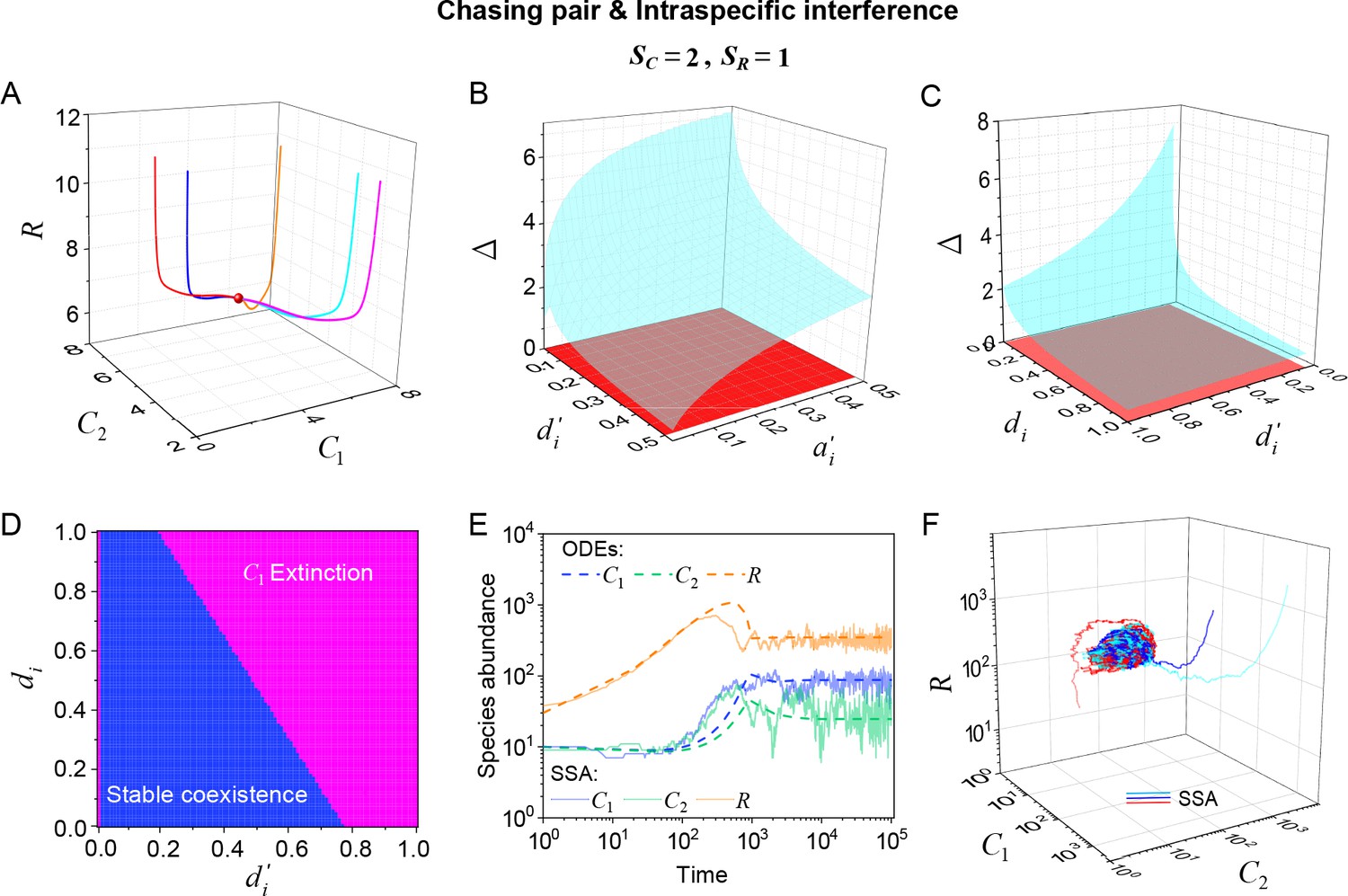
Intraspecific predator interference facilitates species coexistence regardless of stochasticity.
Here, we consider the case of , . (A) A representative trajectory of species coexistence in the phase space simulated with ODEs. The fixed point (shown in red) is stable and globally attractive. (B, C) 3D phase diagrams in the ODEs studies. Here, is the only parameter that varies with the two consumer species, and measures the competitive difference between the two species. The parameter region below the blue surface yet above the red surface represents stable coexistence. The region below the red surface and above represents unstable fixed points (an empty set). (D) An exemplified transection corresponding to the plane in (C). (E) Time courses of the species abundances simulated with ODEs or SSA. (F) Representative trajectories of species coexistence in the phase space simulated with SSA. The coexistence state is stable and globally attractive (see (E) for time courses, SSA results). (A–F) were calculated or simulated from Equations 1, 2 and 4. In (A): , , , , , , , , , , . In (B): , , , , , , , , . In (C, D): , , , , , , , , . In (D): . In (E, F): , , , ,, , , , , , .
Appendix 1—figure 5
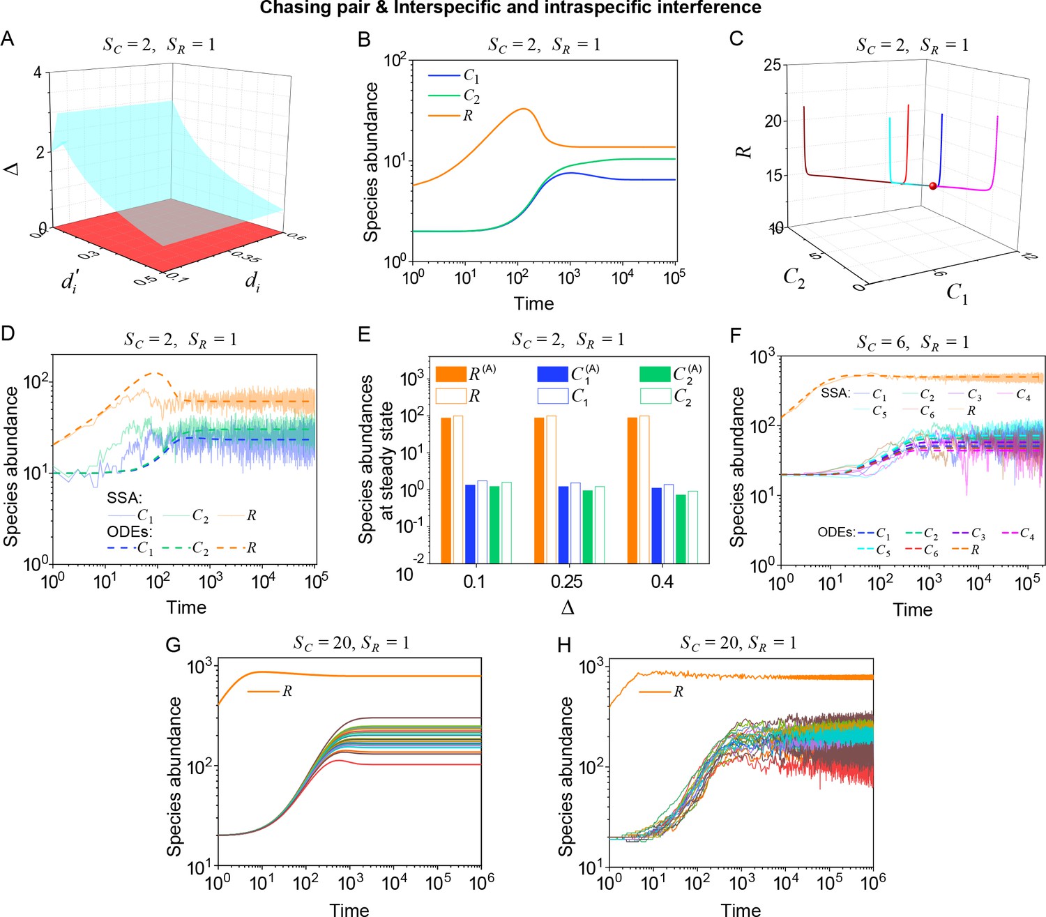
Outcomes of multiple consumers species competing for one resource species involving chasing pairs and intra- and inter-specific interference.
(A–E) The case involving two consumer species and one resource species (, ). Here, is the only parameter that varies with the consumer species (with ), and measures the competitive difference between the two species. (A) A 3D phase diagram. The parameter region below the blue surface yet above the red surface represents stable coexistence, while that below the red surface and above represents unstable fixed points (an empty set). (B) Time courses of the species abundances. Two consumer species may coexist with one type of resources at steady state. (C) Representative trajectories of species coexistence in the phase space. The fixed point (shown in red) is stable and globally attractive. (D) Consumer species may coexist indefinitely with the resources regardless of stochasticity. (E) Comparisons between numerical results and analytical solutions of the species abundances at fixed points. Color bars are analytical solutions while hollow bars are numerical results. The analytical solutions (marked with superscript ‘(A)’) were calculated from Equation S74 and S75. (F–H) Time courses of species abundances in cases involving 6 or 20 consumer species and one type of resources ( or 20, ). All consumer species may coexist with one type of resource at a steady state, and this coexisting state is robust to stochasticity. (A–C, E, G) ODEs results. (D, F) ODEs and SSA results. (H) SSA results. The numerical results in (A–H) were calculated or simulated from Equations 1-4. In (A–C): , , , , , , , , , . In (B–C): , , . In (D): , , , , , , , , , , , , . In (E): , , , , , , , , , , , . In (F): , , , , , , , , , , , , , , , , , . In (G–H): , , , , , , , , , , , , .
Appendix 1—figure 6
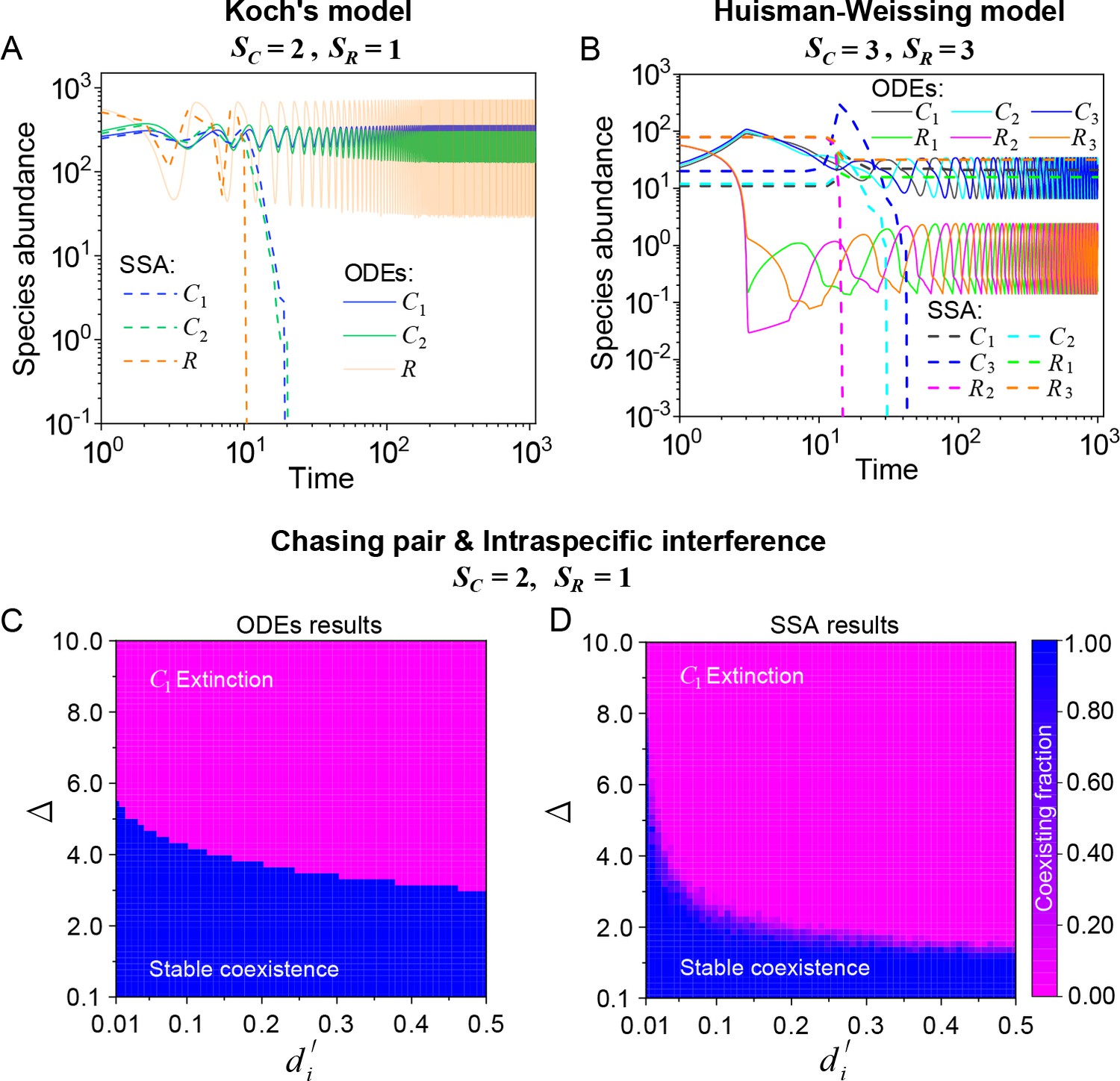
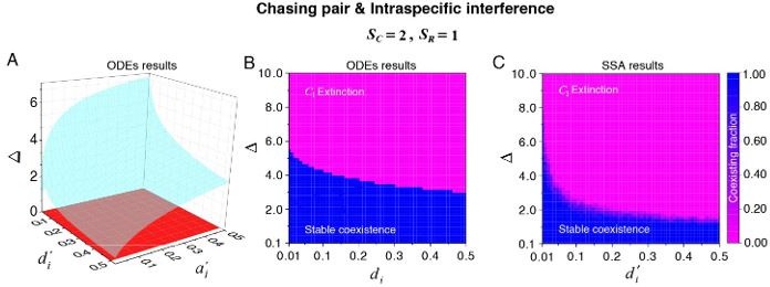
The influence of stochasticity on species coexistence.
(A, B) Stochasticity jeopardizes species coexistence. Koch’s model (Koch, 1974) and Huisman-Weissing model (Huisman and Weissing, 1999) were simulated with SSA using the same parameter settings as their deterministic model. Nevertheless, both cases of oscillating coexistence are vulnerable to stochasticity. See (Koch, 1974) and (Huisman and Weissing, 1999) for the parameters. (C, D) Phase diagrams in the scenario involving chasing pairs and intraspecific interference. Here, and . is the only parameter varying with the consumer species (with ), and represents the competitive difference between the two species. (C) The ODEs results. (D) The SSA results (with the same parameter region as (C)). The species’ coexisting fraction in each pixel was calculated from 16 random repeats. (C) and (D) were calculated from Equations 1, 2 and 4. In (C, D): , , , , , , , , .
Appendix 1—figure 7
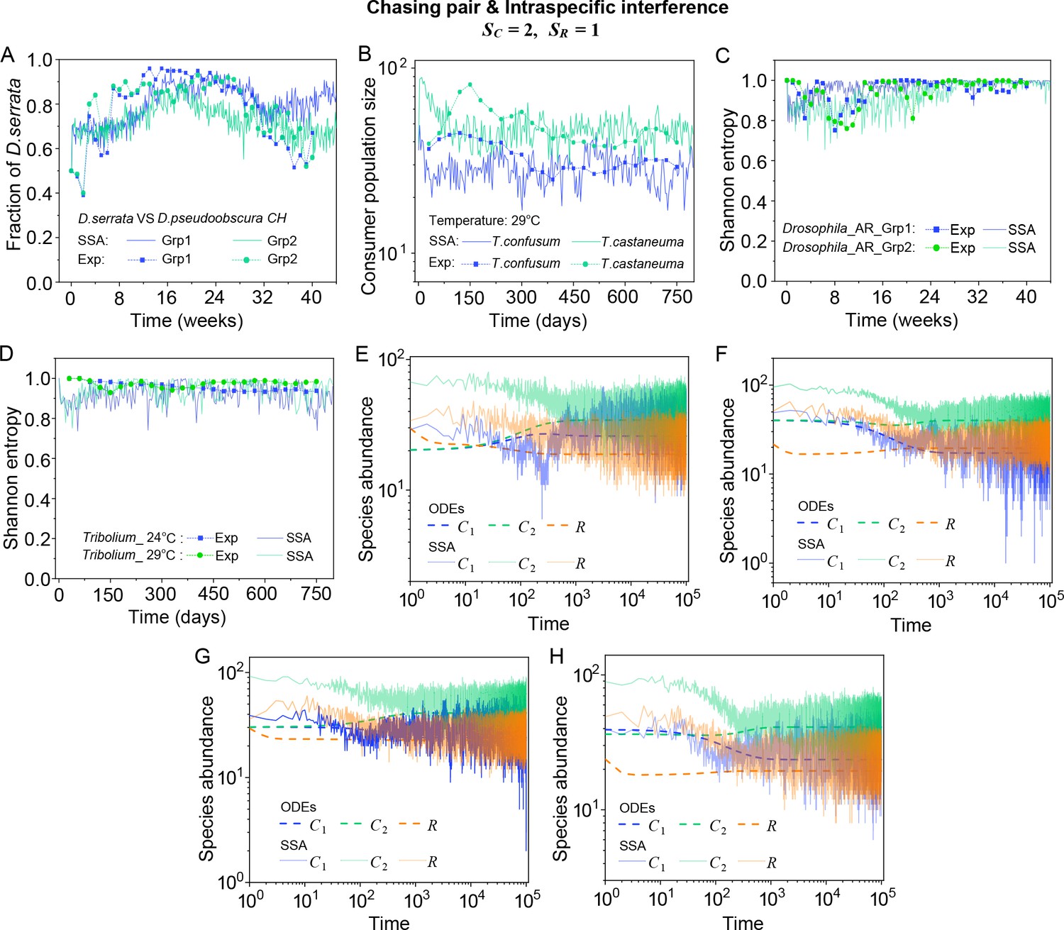
A model of intraspecific predator interference explains two classical experiments that invalidate CEP.
(A) In Ayala’s experiment (Ayala, 1969), two Drosophila species (consumers) coexisted for 40 weeks with the same type of abiotic resources within a laboratory bottle. The time averages () and standard deviation () of the species’ relative abundances for the experimental data or SSA results are: , , , , where the superscript ‘(R)’ represents relative abundances. (B) In Park’s experiment (Park, 1954), two Tribolium species coexisted for 750 days with the same food (flour). The time averages () and standard deviations () of the species’ abundances are: , , , . (A, B) The solid icons represent the experimental data, which are connected by the dotted lines for the sake of visibility. The solid lines stand for the SSA simulation results. (C, D) The Shannon entropies of each time point for the experimental or model-simulated communities shown in (B) and Figure 2D and E. Here, we calculated the Shannon entropies with , where is the probability that a consumer individual belongs to species at the time stamp of . The time averages () and standard deviations () of the Shannon entropies are: , , , , , , , . (E–H) Time courses of the species abundances in the scenario involving chasing pairs and intraspecific interference. The time series in (E–H) correspond to the long-term version of that shown in Figure 2D, Appendix 1—figure 7A, Figure 2E, Appendix 1—figure 7B, respectively. (A, B, F–I) were simulated from Equations 1, 2 and 4. In (A): , , , , , , , , , , . In (B): , , , , , , , , , , . In(A-B): Day (see Appendix 7).
Appendix 1—figure 8
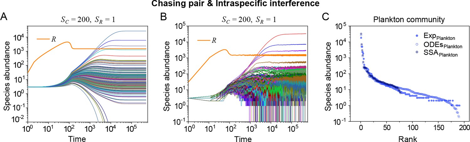
A model of intraspecific interference semi-quantitatively illustrates the rank-abundance curve of a plankton community ().
(A, B) Intraspecific interference enables a wide range of consumers species to coexist with one type of resources. (A) Time courses of the species abundances simulated with ODEs. (B) Time series of the species abundances simulated with SSA (with theh same as parameter settings as (A)). (C) The rank-abundance curve of a plankton community. The solid dots represent the experimental data (marked with ‘Exp’) reported in a recent study (Ser-Giacomi et al., 2018) (TARA_139.SUR.180.2000.DNA), while the hollow dots and those with ‘+’ center are the ODEs and SSA results constructed from timestamp in the time series (see (A) and (B)), respectively. The Shannon entropies of the experimental data and simulation results for the plankton community are: . In the model settings, and . is the only parameter that varies with the consumer species, which was randomly drawn from a Gaussian distribution . Here, μ and σ are the mean and standard deviation of the distribution. The numerical results in (A–C) were simulated from Equations 1, 2 and 4. In (A–C): , , , , , , , , , .
Appendix 1—figure 9
A model of intraspecific interference illustrates the rank-abundance curves across different ecological communities ().
The solid dots represent the experimental data (marked with ‘Exp’) reported in existing studies (Hubbell, 2001; Holmes et al., 1986; Cody and Smallwood, 1996), while the hollow dots and those with ‘+’ center are the ODEs and SSA results constructed from timestamp in the time series (see Appendix 1—figure 10A–G), respectively. In the model settings, , (in (A)), 35 (in (B)) or 45 (in (C)). is the only parameter varying with the consumer species, which was randomly drawn from a Gaussian distribution. The Shannon entropies of the experimental data and simulation results for each ecological community are: , , . In the Kolmogorov-Smirnov (K-S) test, the probabilities (p-values) that the simulation results and the corresponding experimental data come from identical distributions are: , , , , . With a significance threshold of 0.05, none of the p-values suggest there exists a statistically significant difference. The numerical results in (A–C) were simulated from Equations 1, 2 and 4. In (A): , , , , , , , , , . In (B): , , , , , , , , , . In (C): , , , , , , , , , .
Appendix 1—figure 10
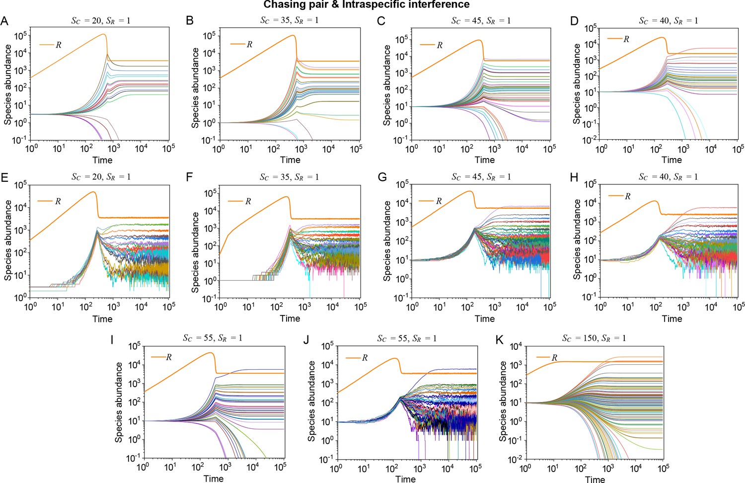
Time courses of the species abundances in the scenario involving chasing pairs and intraspecific interference.
The time series in (A, E), (B, F), (C, G), (D, H), (I, J) and (K) correspond to that shown in Appendix 1—figure 9A–C, Figure 3D (bat), Figure 3D (lizard) and Figure 3C (butterfly), respectively.
Appendix 1—figure 11
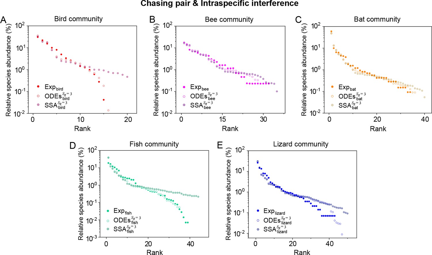
A model of intraspecific interference illustrates the rank-abundance curves across different ecological communities ().
The solid dots represent the experimental data (marked with ‘Exp’) reported in existing studies (Hubbell, 2001; Holmes et al., 1986; Cody and Smallwood, 1996; Clarke et al., 2005), while the hollow dots and those with ‘+’ center are the ODEs and SSA results constructed from timestamp in the time series (see Appendix 1—figure 13), respectively. In the model settings, , (in (A)), 35 (in (B)), 40 (in (C)), 45 (in (D)) or 50 (in (E)). is the only parameter varying with the consumer species, which was randomly drawn from a Gaussian distribution. The Shannon entropies of the experimental data and simulation results for each ecological community are: , , , , . In the K-S test, the p-values that the simulation results and the corresponding experimental data come from identical distributions are: , , , , , , , , , . With a significance threshold of 0.05, none of the p-values suggest there exists a statistically significant difference. The numerical results in (A–E) were simulated from Equations 1, 2 and 4. In (A–E): , , . In (A): , , , , , , , , , , , . In (B): , , , , , , , , , , , . In (C): , , , , , , , , , , , . In (D): , , , , , , , , , , , . In (E): , , , , , , , , , , , .
Appendix 1—figure 12
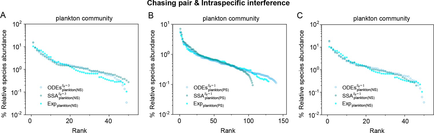
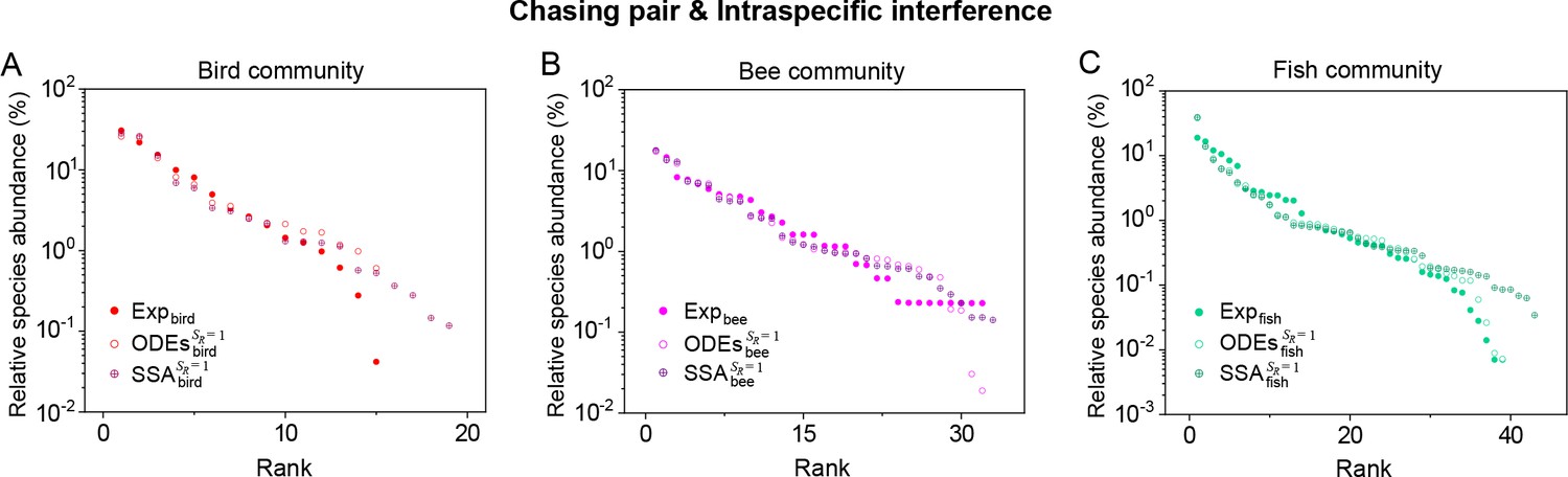
A model of intraspecific interference illustrates the rank-abundance curves across different plankton communities ().
The solid dots represent the experimental data (marked with ‘Exp’) reported in a recent study (Fuhrman et al., 2008), while the hollow dots and those with ‘+’ center are the ODEs and SSA results constructed from timestamp in the time series (see Appendix 1—figure 13), respectively. The plankton community data were obtained separately from the Norwegian Sea (NS) and Pacific Station (PS). In the model settings, (in (B, C)), 3 (in (A)); (in (A, C)), 150 (in (B)). is the only parameter varying with the consumer species, which was randomly drawn from a Gaussian distribution. The Shannon entropies of the experimental data and simulation results for each plankton community are: for , for . In the K-S test, the p-values that the simulation results and the corresponding experimental data come from identical distributions are: , for , , for . With a significance threshold of 0.05, none of the p-values suggest there exists a statistically significant difference. The numerical results in (A–C) were simulated from Equations 1, 2 and 4. In (A): , , , , , , , , , , , , , , . In (B): , , , , , , , , , , . In (C): , , , , , , , , , .
Appendix 1—figure 13
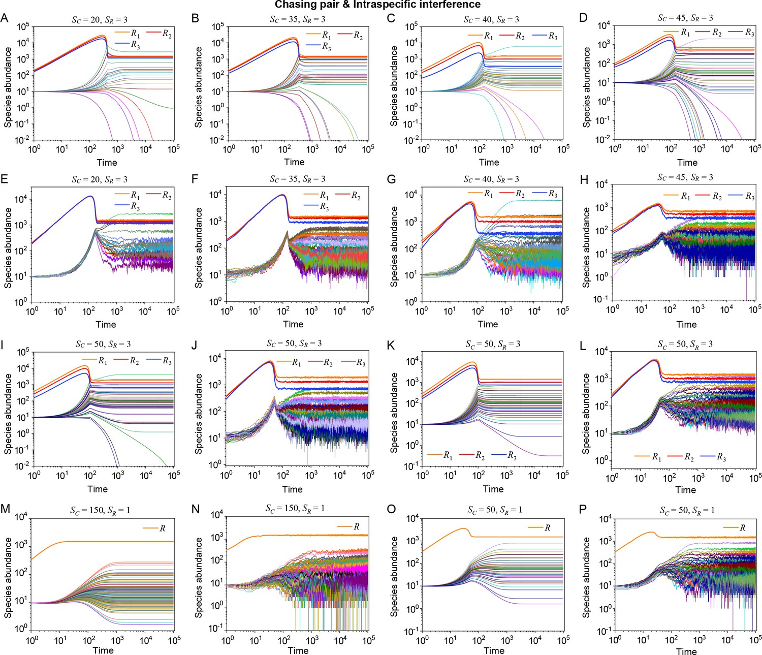
Time courses of the species abundances in the scenario involving chasing pairs and intraspecific interference.
The time series in (A, E), (B, F), (C, G), (D, H), (I, J), (K, L), (M, N) and (O, P) correspond to that shown in Appendix 1—figure 11A–E and Appendix 1—figure 12A–C, respectively.
Appendix 1—figure 14
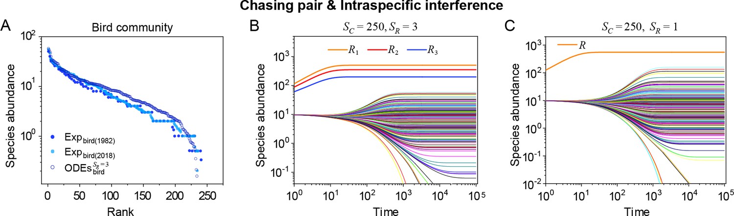
A model of intraspecific interference illustrates the rank-abundance curve of a bird community ().
(A) The rank-abundance curve. The solid dots represent the bird community data (marked with ‘Exp’) collected longitudinally within the same Amazonian region in 1982 (blue) and 2018 (cyan) (Terborgh et al., 1990; Martínez et al., 2023). The hollow dots are the ODEs results constructed from timestamp in the time series (see (B)). (B) Time courses of the species abundances simulated with ODEs. In the model settings, and is the only parameter varying with the consumer species, which was randomly drawn from a Gaussian distribution. The Shannon entropies of the experimental data and simulation results for the bird community are . In the K-S test, the p-values that the simulation results and the corresponding experimental data come from identical distributions are: , . With a significance threshold of 0.05, none of the p-values suggest there exists a statistically significant difference. (C) Time courses of the species abundances simulated with ODEs corresponding to Figure 3C (bird), and the simulation parameters are the same as Figure 3C (bird). The numerical results in (A–C) were simulated from Equations 1, 2 and 4. In (A, B): , , , , , , , , , , , , , .
Appendix 1—figure 15
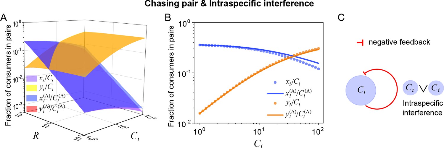
Intraspecific interference results in an underlying negative feedback loop and thus promotes biodiversity.
(A, B) The fraction of consumer individuals engaged in pairwise encounter. Here, and . xi represents , and yi represents and stand for the fractions of consumer individuals within a chasing pair and an interference pair, respectively. The numerical results were calculated from Equation S55, while the analytical solutions (marked with superscript ‘(A)’) were calculated from Equation S59. The orange surface in (A) is an overlap of the red and yellow surfaces. (C) The formation of intraspecific interference results in a self-inhibiting negative feedback loop. In (A, B): . In (B): .
Author response image 1

Shannon Entropies of the experimental data and SSA results in Fig.
2D-E, redrawn from Appendix-fig. 7C-D.
Author response image 2
The parameter region for two consumer species coexisting with one type of abiotic resource species (SC = 2 and SR = 1).
(A) The region below the blue surface and above the red surface represents stable coexistence of the three species at constant population densities. (B) The blue region represents stable coexistence at a steady state for the three species. (C) The color indicates (refer to the color bar) the coexisting fraction for long-term coexistence of the three species. Figure redrawn from Appendixfigs. 4B, 6C-D.
Author response image 3

Bifurcation analyses for the separate rate d’i and escape rate di (i = 1, 2) of our model in the case of two consumer species competing for one abiotic resource species (SC = 2 and SR = 1).
(A) A 3D representation: the region above the blue surface signifies competitive exclusion where C1 species extinct, while the region below the blue surface and above the red surface represents stable coexistence of the three species at constant population densities. (B) A 2D representation: the blue region represents stable coexistence at a steady state for the three species. Figure redrawn from Appendix-fig. 4C-D.
Tables
Appendix 1—table 1
Illustrations of symbols in our generic model of pairwise encounters.
| Symbols | Illustrations |
|---|---|
| The total population of consumer species . | |
| The total population of resource species . | |
| The freely wandering population of consumer species . | |
| The freely wandering population of resource species . | |
| Chasing pairs formed between individuals from species and , i.e. . | |
| Intraspecific interference pairs formed between individuals from species , i.e. . | |
| Interspecific interference pairs formed between individuals from species and , i.e., . | |
| The upper distance criterion for forming a chasing pair. | |
| The upper distance criterion for forming an interference pair. | |
| The motility speed of consumer species . | |
| The motility speed of resource species . | |
| The number of consumer species. | |
| The number of resource species. | |
| The encounter rate between a consumers and a resource. | |
| The escape rate within a chasing pair. | |
| The capture rate within a chasing pair. | |
| The encounter rate among consumer individuals. | |
| The separation rate within an interference pair. | |
| The mass conversion ratio from resource to . | |
| The mortality rate of species . | |
| The steady-state population abundance of resources species in the absence of consumers. | |
| The external resource supply rate of species . | |
| The intrinsic growth rate of species for biotic resources (unused in all analyses). | |
| The function describing the population dynamics of resource species . | |
| The length of the 2-D square system where species coexist. | |
| We count as , where ”(+)” signifies gaining biomass from resources. | |
| The velocity of an individual of species . | |
| The velocity of an individual of species . | |
| The angle between and . | |
| The relative velocity between a consumer and a resource. | |
| The relative speed between a consumer and a resource. | |
| The concentration of species . | |
| The concentration of species . | |
| The concentration of the freely wandering . | |
| The concentration of the freely wandering . |
-
For all the symbols in Appendix 1—tables 1 and 2, the subscript ‘’ is omitted if , and the subscript ‘’ is omitted if .
Appendix 1—table 2
Illustrations of other symbols used in our manuscript.
| Symbols | Illustrations/Definitions |
|---|---|
| The functional response. | |
| The searching efficiency. | |
| A random number sampled from a uniform distribution. | |
| The uniform distribution. | |
| A Gaussian distribution with a mean of μ and a standard deviation of σ. | |
| An equal sign for equations defining the symbol on the left-hand side. | |
| The competitive difference between two consumer species, defined as . | |
| The supremum of the competitive difference tolerated for species coexistence. | |
| A short time interval. | |
| The probability that a consumer individual of the ecological community belongs to species . | |
| , | The p-value assessing the similarity of simulation results and experimental data. |
| The Shannon entropy: . | |
| The time average of an arbitrary quantity . | |
| The standard deviation of an arbitrary quantity . | |
| The expectation of a random variable . | |
| The parameter that sets the time scale of a system. | |
| . | |
| . | |
| . | |
| . | |
| . | |
| , , | , , . |
| The discriminant of Equation S13. | |
| , | , . |
| , , | , , . |
| , | , . |
| The handling time in the B-D model. | |
| The wasting time in the B-D model. | |
| Expression of using , , and in Equation S33 involving intraspecific interference, see Equation S37. | |
| . | |
| , see Equations S33 and S38. | |
| , | , . |
| . | |
| , | , . |
| Expression of using , , and in Equation S61 involving interspecific interference, see Equation S64. | |
| , see Equation S61 and S65. | |
| , | , . |
| . | |
| . |
Additional files
Download links
A two-part list of links to download the article, or parts of the article, in various formats.
Downloads (link to download the article as PDF)
Open citations (links to open the citations from this article in various online reference manager services)
Cite this article (links to download the citations from this article in formats compatible with various reference manager tools)
Intraspecific predator interference promotes biodiversity in ecosystems
eLife 13:RP93115.
https://doi.org/10.7554/eLife.93115.3


