Reversions mask the contribution of adaptive evolution in microbiomes
- Institute for Medical Engineering and Sciences, Massachusetts Institute of Technology, United States
- Department of Civil and Environmental Engineering, Massachusetts Institute of Technology, United States
- Broad Institute of MIT and Harvard, United States
- Ragon Institute of MGH, MIT and Harvard, United States
Figures
Figure 1 with 3 supplements
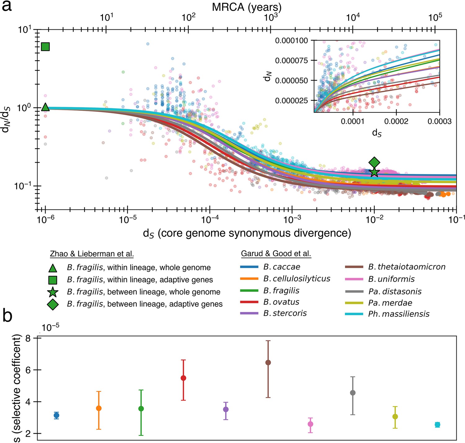
The previously proposed explanation for the time dependence of dN/dS is weak purifying selection.
(a) Time signature of dN/dS as depicted by data points derived from the studies by Garud et al., 2019 and Zhao et al., 2019. Each dot represents a pairwise comparison between the consensus sequence from two gut microbiomes as computed by Garud et al., 2019, using only the top 10 species based on the quality of data points (see ‘Methods’). Where the high initial value of dN/dS begins to become the low asymptotic value of dN/dS occurs at approximately . Fit lines were derived from these points using Equation 4 to depict the trend. The median R2 is 0.81 (range 0.54–0.94). Corresponding data from Zhao et al., 2019 confirms these observed trends, demonstrating high levels of dN/dS at short timescales and low levels at longer timescales. Adaptive genes are from Zhao et al., 2019 and are defined as those that have high dN/dS values in multiple lineages. Insets: dN vs. dS on a linear scale. Note that the data was fit to minimize variance in the logarithmic scale, not the linear scale, so the fit is not expected to be as good for the inset. See Figure 1—figure supplement 1 for minimizing variance on a linear scale. See Figure 1—figure supplement 2 for all species on separate panels. (b) Values of s from the output of 999 standard bootstrap iterations of curve fitting, conducted with replacement, demonstrate that only small values of the average selective coefficient can fit the data.
Figure 1—figure supplement 1
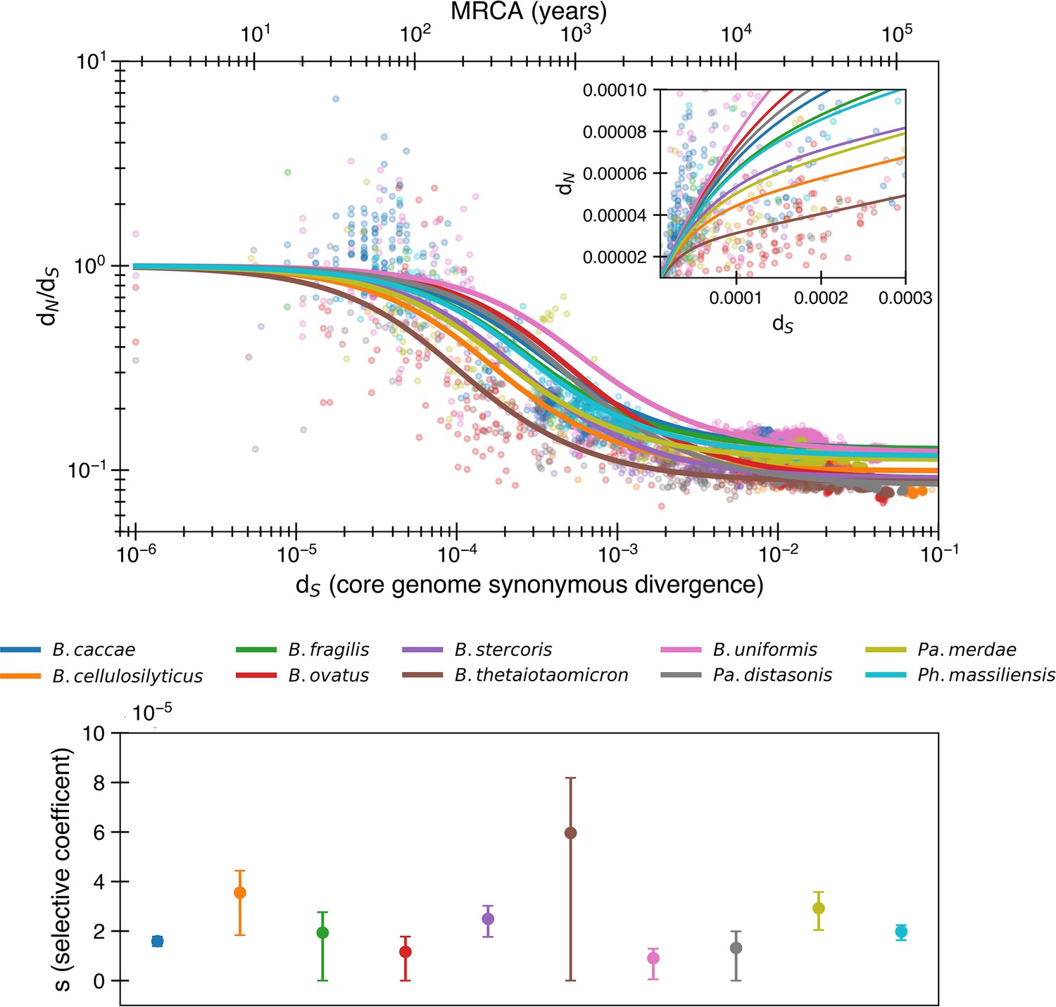
The purifying selection model predicts even weaker purifying selection when fitting to nonlogarithmic dN/dS.
Equivalent to Figure 1, except the fit is determined by minimizing variance in dN/dS rather than logarithmic dN/dS. In this fit, s values tend to be even smaller, with a median of 2.0 × 10⁻⁵. The median R2 = 0.64 (range 0.07–0.88).
Figure 1—figure supplement 2
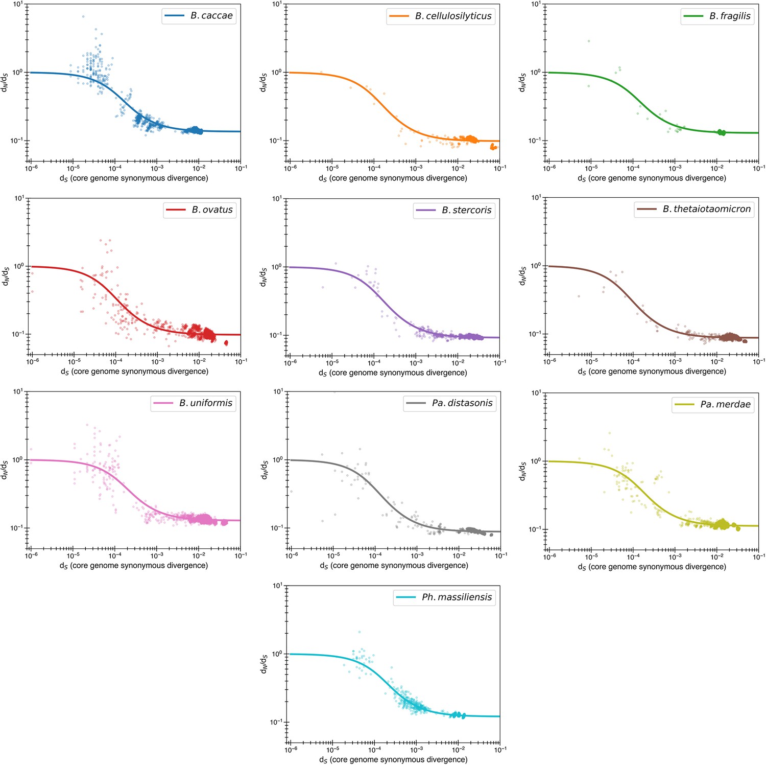
Purifying selection model fits by individual species.
Figure 1—figure supplement 3
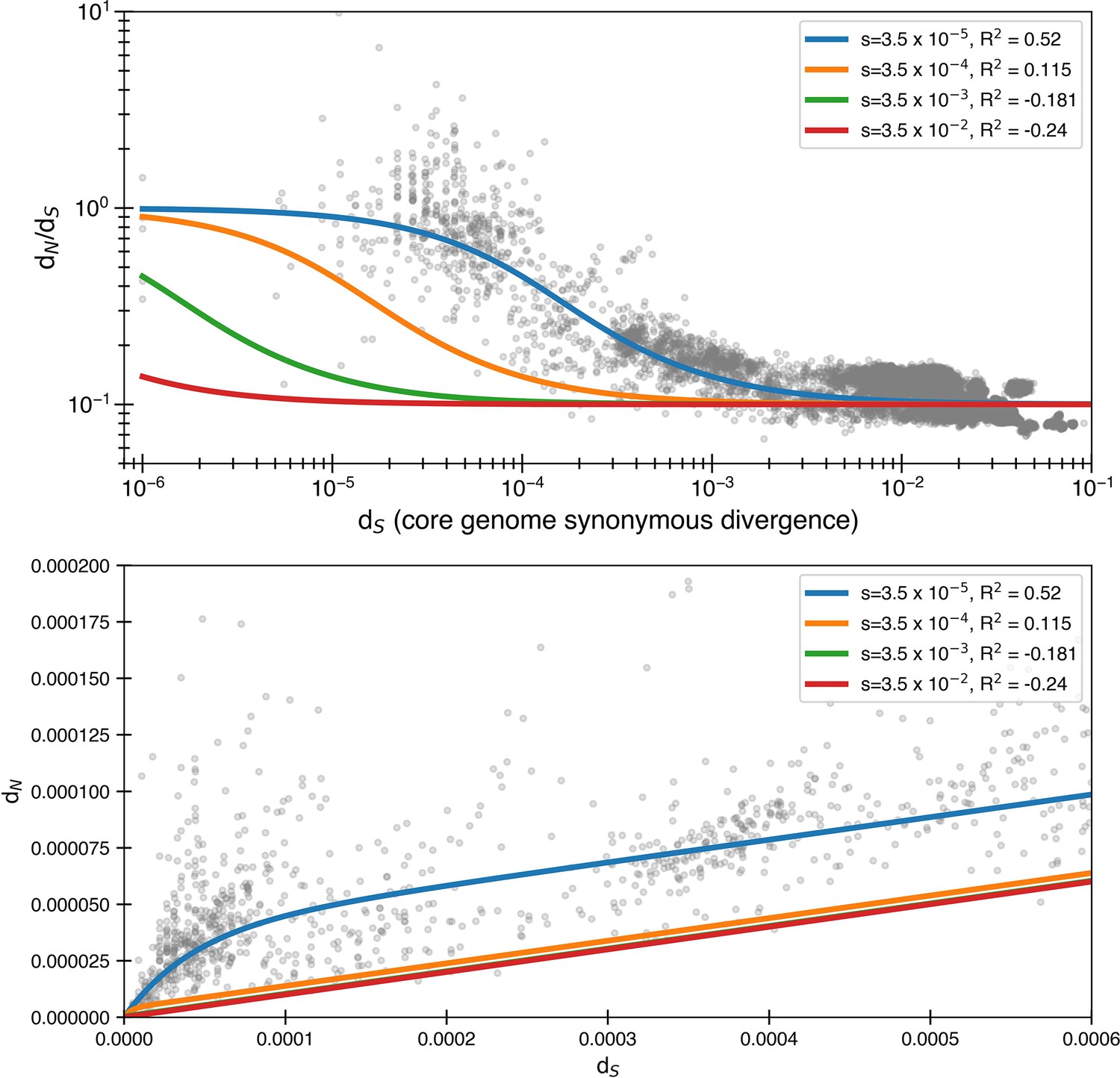
Larger selective coefficients rapidly lose explanatory power.
Here, we use Equation 4 to once again fit the data. We still use but use alternate values of s. We see that significantly larger, though still relatively small, levels of purifying selection have essentially no ability to explain the data. is for minimizing the logarithmic variance.
Figure 2 with 4 supplements
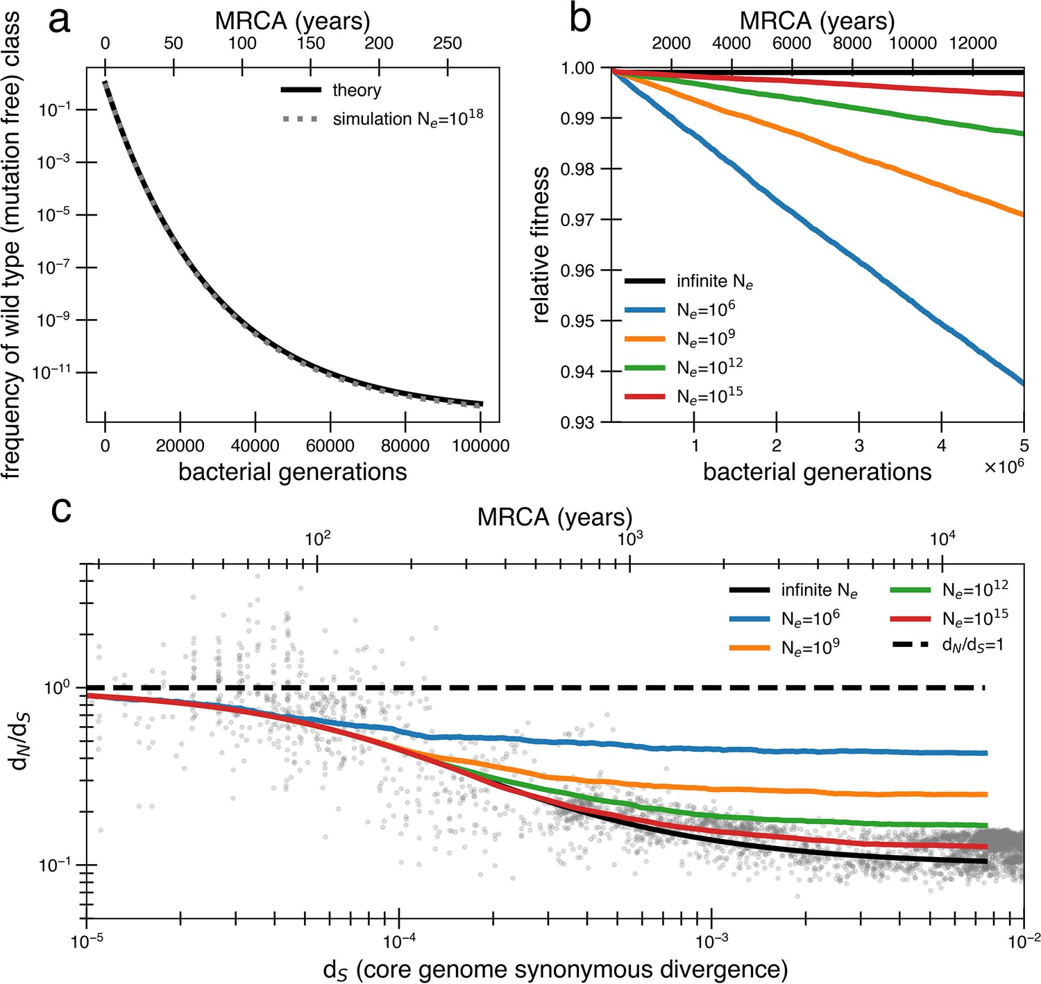
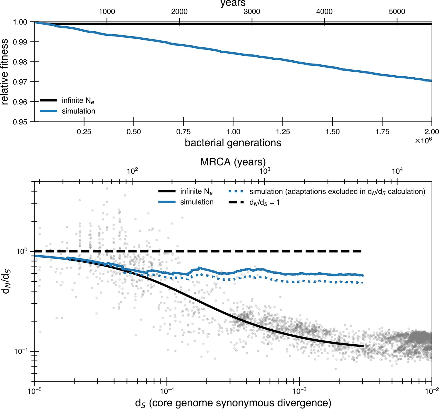
Models of extremely weak purifying selection that can fit the data suffer from mutation accumulation and fitness decay.
(a) The temporal dynamics of the least-loaded class in a large population under the purifying selection model. The black line represents the predicted frequency of the wild-type (mutation-free) class over time. The simulation curve shows simulation results assuming constant purifying selection in an exceptionally large effective population size (Ne = 1018; see text for a discussion of population size) under a slightly modified Wright–Fisher model (‘Methods’). (b) As a consequence of the loss of the least-loaded class, fitness declines in finite populations over time. Colored lines indicate simulations from various effective population sizes with mutations of constant selective effect. The deleterious mutation rate in the simulation is 1.01 × 10⁻³ per genome per generation. (c) Using the same simulations as in panel (b), we see that realistic global effective population sizes fail to fit the dN/dS curve, with different asymptotes. The black line denotes the infinite population theoretical model, and the colored lines indicate increasing effective population sizes, which change the strength of genetic drift in the simulations. Larger values of s and models in which all mutations are deleterious cannot fit the data (Figure 2—figure supplement 1, Figure 2—figure supplement 2). Generations are assumed to occur once every day.
Figure 2—figure supplement 1
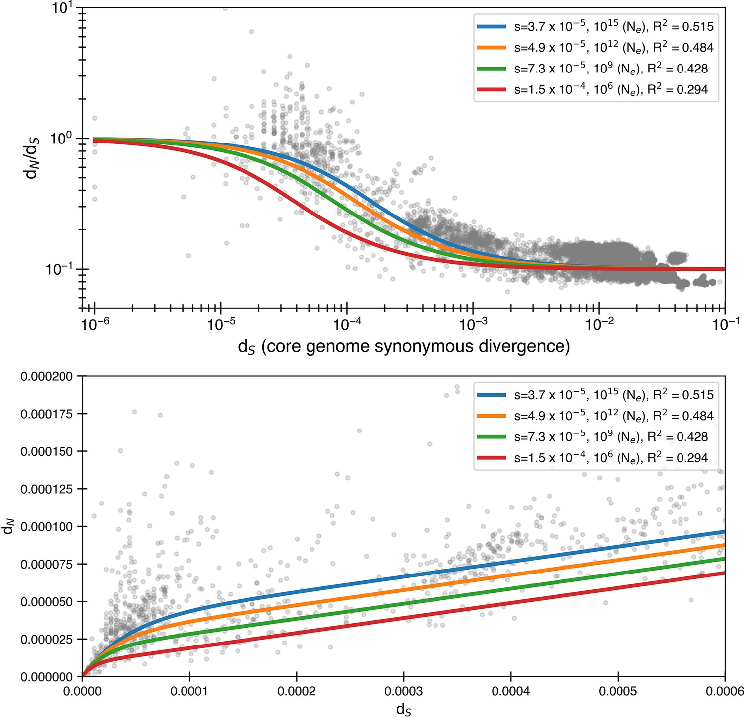
Larger selective coefficients that can prevent mutation accumulation in simulations lead to less optimal data fit.
We first calculate the smallest possible s values (as estimated from Equation 5) that will not lead to mutation accumulation for a given effective population size and the corresponding fits. The core genome size is assumed to be 1,500,000 nucleotides. Once again, we use Equation 4 to fit the data and use .
Figure 2—figure supplement 2
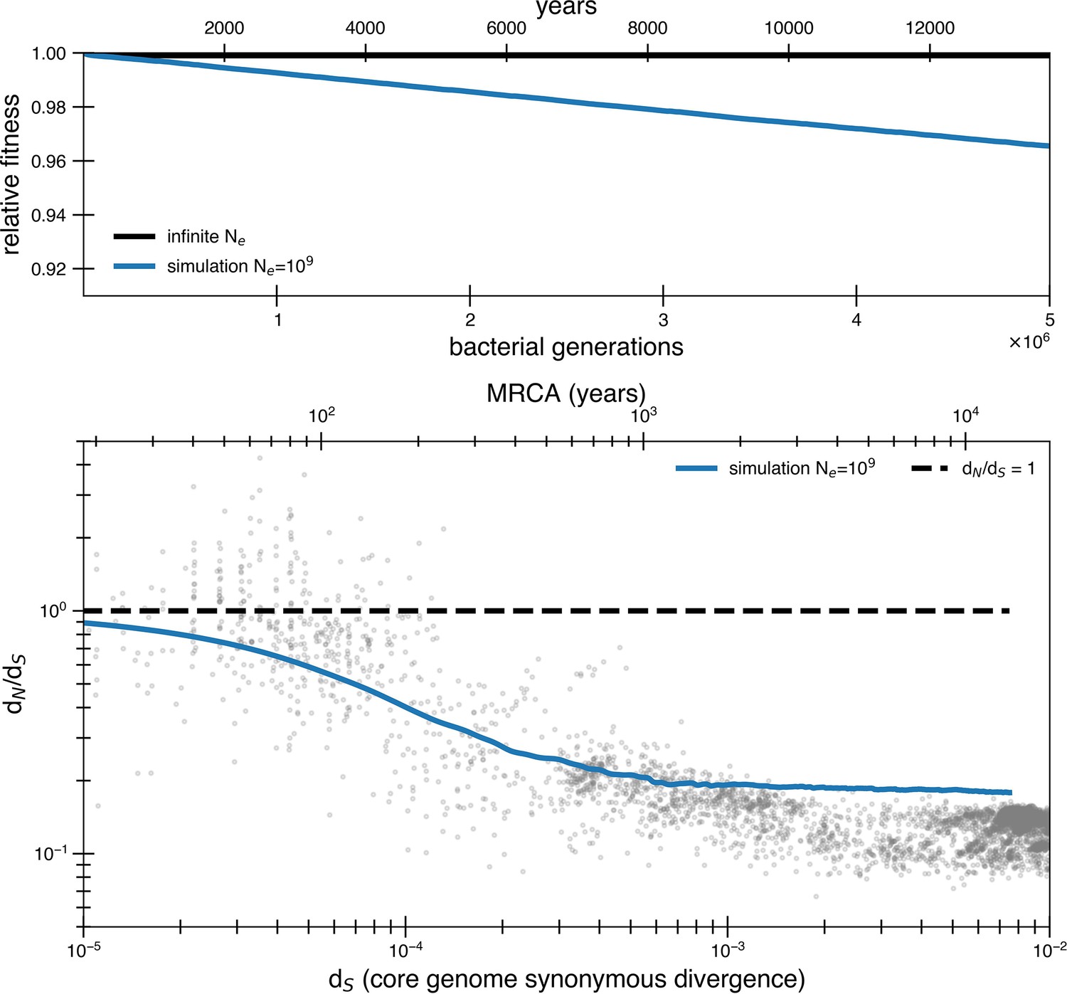
Even assuming all mutations are deleterious suggests a higher asymptotic dN/dS.
A purifying selection simulation as in Figure 2, except that all mutations are assumed to be weakly deleterious (s = 3.5 × 10⁻⁵) rather than just 90%. In other words, rather than the standard deleterious mutation rate of 1.01 × 10⁻³ mutations per genome per generation, the mutation rate is now 1.13 × 10⁻³ mutations per genome per generation. With an effective population size of 109, mutations still occur so quickly as to raise the asymptote above the data. Furthermore, all of these mutations contributing to the asymptotic dN/dS are deleterious rather than neutral, furthering the problem of Muller’s ratchet.
Figure 2—figure supplement 3
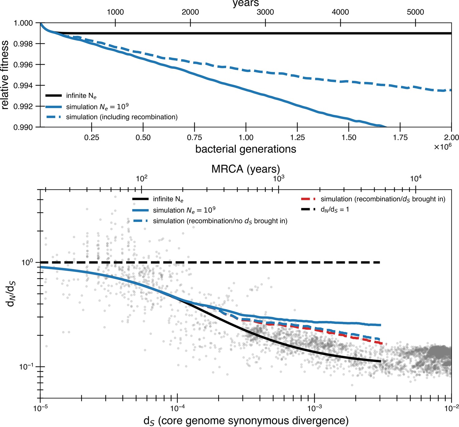
High rates of recombination are unlikely to rescue a model of weak purifying selection.
A purifying selection simulation with a population of 109 with and without recombination. To simulate the potential for recombination to purge deleterious mutations, we assume a 2.5 × 10⁻⁷ chance per codon per generation of return to the ancestral state (500 times the basal mutation rate, dotted blue line), which brings alongside it a linked synonymous mutation. This would represent recombination bringing in fragments of 100 bp in length from a genome with dS = 0.01. All other assumptions are the same as the continuous selection simulations in Figure 2. While recombination does allow more fit genotypes to arise, their selective advantage is quite small, and time to sweep is still slower than mutation accumulation. Recombination is more effective at purging deleterious alleles when many deleterious mutations are present, but this occurs at a longer timescale than the actual drop off of dN/dS values. We also include a variant where recombination events revert deleterious mutations without linked synonymous mutations. In this model, we have only included recombination events that revert deleterious mutations and chosen not to explicitly model cases of neutral recombination. High levels of neutral recombination with distant organisms would result in closely related organisms having dN/dS significantly less than 1 and would not fit the data without significant adaptation.
Figure 2—figure supplement 4
Transmission bottlenecks and adaptation further complicate purifying selection.
Results of a simulation with purifying selection that takes into account transmission bottlenecks and the possibility of adaptation. The simulation is meant to represent a potential transmission chain from gut to gut. This simulation is a modified version of the simulation used for the reversion model (see ‘Methods’). Only forward mutations are available when beneficial mutations arrive () and deleterious mutations arrive at a rate of 1.01 × 10⁻³ mutations per genome with a selective disadvantage of s = 3.5 × 10⁻⁵. The census size in an individual gut is 1010. We choose very conservative values for adaptation rate, bottleneck size, and bottleneck frequency to show how even small levels of these dynamics strongly influence results. Transmission bottlenecks happen on average every 100,000 generations. The population is bottlenecked to 1000 members upon transmission. Beneficial selective pressures are released on average every 8400 generations. Multiple beneficial pressures can occur together (the number released at a time is a Poisson random variable of mean 1). This rate of beneficial mutation does not contribute much to dN/dS on its own as seen from the dotted line where adaptations are excluded in the dN/dS calculation. However, both of these scenarios drastically increase the rate of mutation accumulation and the asymptotic dN/dS. The reversion model can prevent this from occurring with 10 times the amount of adaptation and transmission.
Figure 3 with 2 supplements
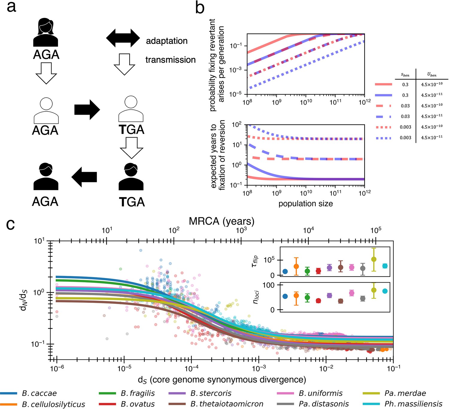
Locally adaptive mutations and subsequent reversions can explain the decay of nonsynonymous mutations.
(a) Cartoon schematic depicting a potential reversion event within a single transmitted lineage of bacteria. The color of each individual indicates a different local adaptive pressure. Closed arrows represent mutation while open arrows indicate transmission. (b) Reversions become increasingly likely at larger population sizes and are nearly guaranteed to occur and fix within 1–10 years when strongly beneficial in gut microbiomes. The probability of revertant arising and fixing (top panel) is calculated as , and the expected time to fixation of reversion (bottom panel) is calculated as ( per generation). Generation times are assumed to be 1 day. Note that the mutation rate does not affect time to fixation much when Ne is large. Here, we assume no clonal interference or bottlenecks, though simulations do take these processes into account. See Appendix 1, Section 2.2 for derivation. Each line type displays a different selective advantage coefficient. (c) The adaptive reversion model can fit the data. Each colored line shows the fit for a different species. The median R2 = 0.82 (range 0.54–0.94). Fit minimizes logarithmic variance. See Figure 3—figure supplement 1 for alternative fitting linear variance. See Figure 3—figure supplement 2 for species individually. Insets: fit parameters for , the average number of generations for a given environmental pressure to switch directions and , the average number of sites under different fluctuating environmental pressures. The scale of the y-axis is linear. Confidence intervals are from 999 bootstrapped resamples.
Figure 3—figure supplement 1
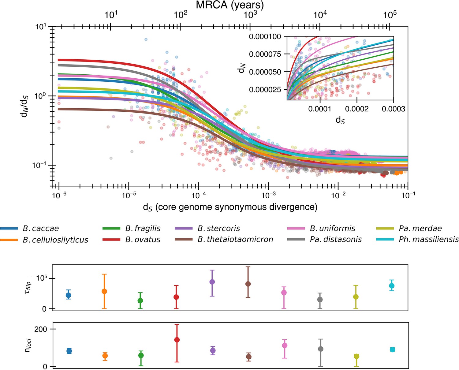
Potential for even more adaptation if fitting nonlogarithmic dN/dS.
Results of fitting the reversion model (Equation 8) to minimize dN/dS rather than logarithmic dN/dS. This implies a potential longer time to switch for a given selective pressure (median ) and an increased number of loci undergoing fluctuating selection (median ). The median R2 = 0.72 (range 0.11–0.88).
Figure 3—figure supplement 2
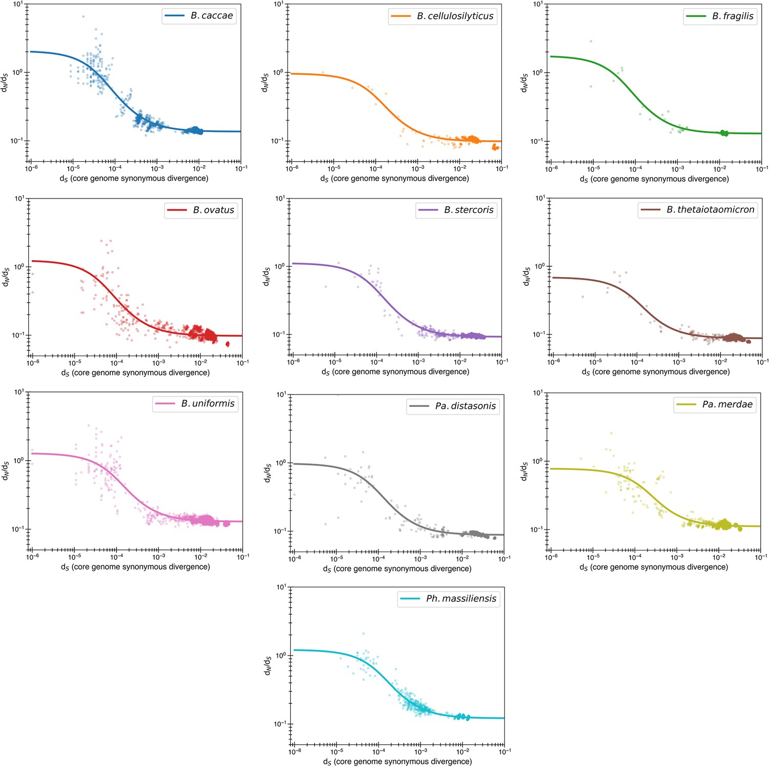
Reversion model fits by individual species.
Content of Figure 3b, with each species now given its own panel. One species of note is B. caccae, which appears to have initial dN/dS values >1, which can now be fit with the reversion model (see Figure 1—figure supplement 2 for comparison with purifying model).
Figure 4 with 3 supplements
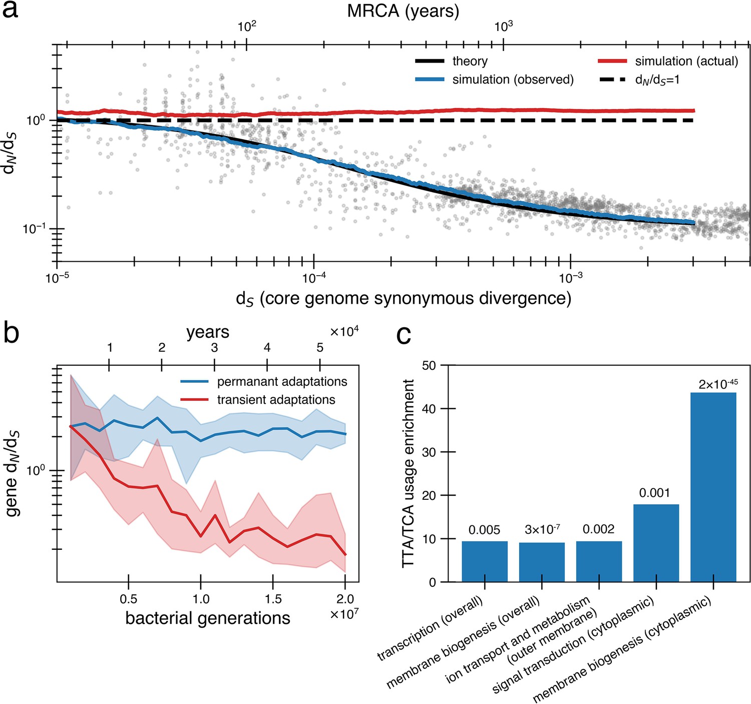
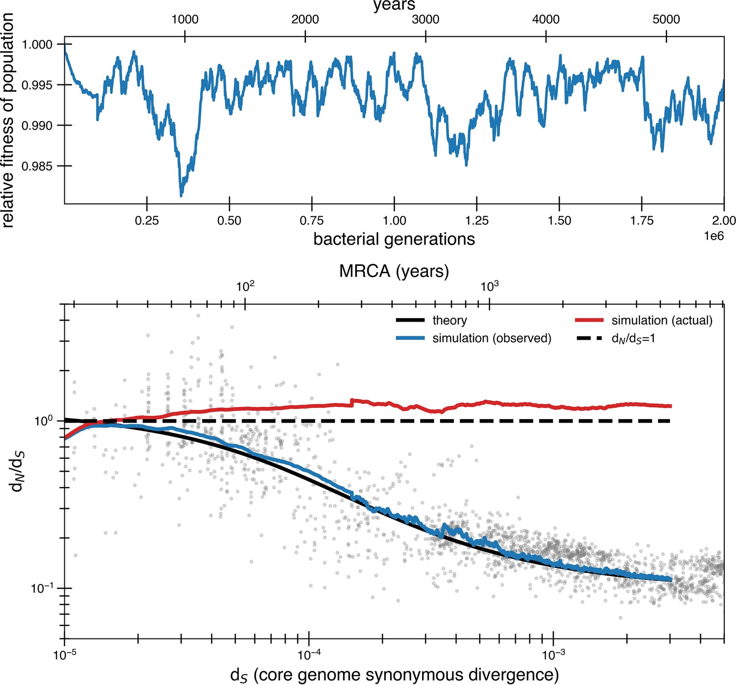
Under a model of reversion, the apparent dN/dS on long timescales underestimates the extent of adaptive evolution.
(a) The reversion model successfully fits the data in simulations. We simulate a population of size 1010 that has a bottleneck to size 10 on average every 10,000 generations (~27 years or a human generation [Wang et al., 2023] given a bacterial generation a day), with one adaptive pressure () occurring on average every 840 generations independently of bottlenecks (see Figure 4—figure supplement 1 for an alternative where bottlenecks and selection are correlated). New pressures either require forward mutations (which can be acquired at a rate of 1.1 × 10⁻⁸ per available locus per generation) or reversions (which can be acquired at a rate of 4.5 × 10⁻¹⁰ per available locus per generation), the balance of which depends on the history of pressures on the tracked genome (i.e., more past forward pressures implies more potential future reverse pressures). Based on the best fit to the data, we use . Deleterious mutations occur at a rate of 1.01 × 10⁻³ mutations per genome and have and can themselves be reverted. More details on the simulation can be found in ‘Methods’. Each curve represents the average of 10 runs; the blue line shows the observed pairwise dN/dS while the red line includes adaptive mutations and reversions. The theory line is the result of Equation 8. Observable dN/dS decays because of reversion, while the actual dN/dS of mutations that occurred is >1 when taking into account both forward and reverse mutations. (b) PAML (Yang, 2007) cannot detect true dN/dS in a given gene in the presence of adaptive reversions. Both lines are dN/dS as calculated by PAML on a simulated gene phylogeny. In the permanent adaptations simulation (blue), adaptive mutations are acquired simply and permanently. In the transient adaptations simulation (red), only more recent mutations will be visible while older mutations are obscured (‘Methods’). Line is the average of 10 simulated phylogenies and shaded regions show the range. (c) Categories of genes in the Bacteroides fragilis genome (NCTC_9343) enriched for stop-codon adjacent codons (TTA and TCA) relative to the expectation from the rest of the genome (‘Methods’). The use of these codons suggests these sequences may have recently had premature stop codon mutations. p-Values are displayed above bars and were calculated using a one-proportion Z-test with Bonferroni correction. See ‘Methods’, Supplementary file 1, and Supplementary file 2 for more details.
Figure 4—figure supplement 1
Effect of correlating mutations with bottleneck has little impact on the fit.
Same parameters as simulation from Figure 4a but rather than have new pressures occur independently of bottlenecks, they occur concurrently. To have an overall average of one beneficial mutation every 840 generations, an average of 11.9 mutations (Poisson with mean 11.9) occur every bottleneck, which occurs on average every 10,000 generations. The most noticeable difference is greater variability at low synonymous divergence values. The first 100,000 generations is the average of 50 simulations while subsequent parts of the curve consist of only 5 simulations to save on computing time (hence the slight spike).
Figure 4—figure supplement 2
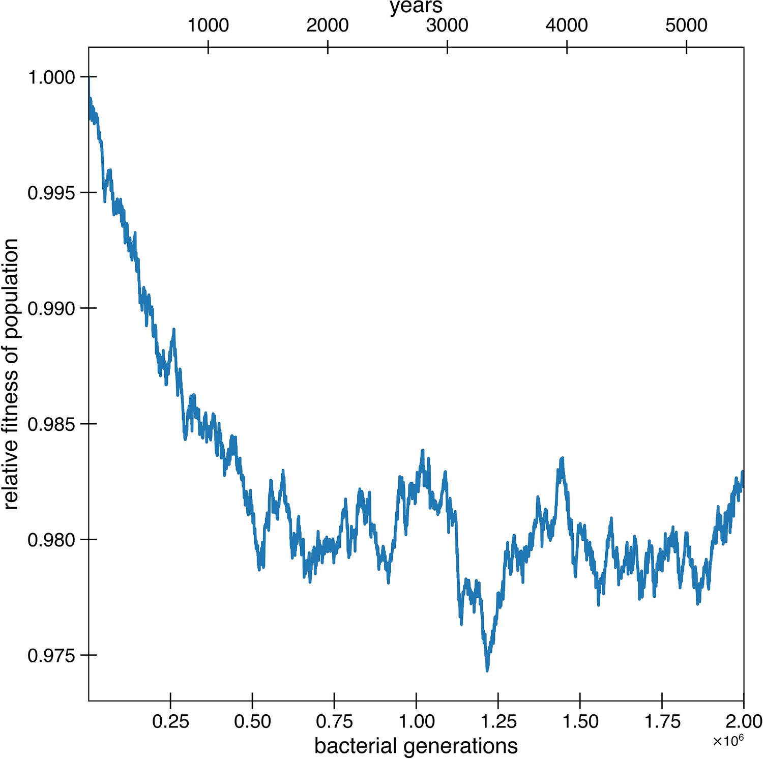
Deleterious hitchhikers are reverted over time, preventing fitness decay.
Besides for reversions potentially occurring due to strong environmental pressures, reversions can also occur because of the fixation of deleterious hitchhikers. These results are from the simulations of Figure 4a, where deleterious mutations occur at a rate of 1.01 × 10⁻³ per genome per generation and with a selective disadvantage of s = 0.003. Deleterious mutations are allowed to hitchhike, and reversions of these deleterious mutations are also permitted. Adaptive mutations and reversions are not counted in relative fitness. The curve is the average of 10 simulations.
Figure 4—figure supplement 3
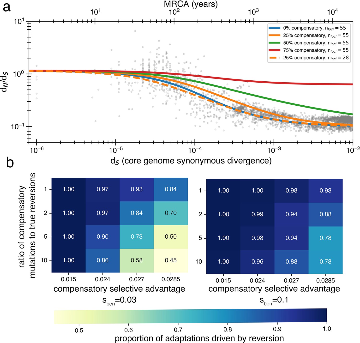
Inclusion of compensatory mutation in the reversion model shows that dN/dS still decays provided reversion occurs at reasonable rates.
(a) Using a Markov chain (see Appendix 1, Section 3.2), we calculate the theoretical values of , and thus dN/dS decay, under varying assumptions about the rate at which compensatory mutations win over true reversions. While compensatory mutations do slow the rate at which dN/dS decays (relative to no compensatory mutations) if reversions are more likely than compensatory mutations, a decay will be observed. Reducing the number of loci can correct for delayed decay from compensatory mutations. (b) The likelihood of true reversion vs. compensatory mutations (treated as mutually exclusive) under different parameter regimes as determined from simulations. Simulations are performed the same as those displayed in Figure 4 and described in the ‘Methods’ section for the reversion model (same population size, bottlenecks, loci, arrival of pressures, mutation rates), except now there is an additional compensatory category that can be used to satisfy an adaptation to a reverse pressure and has a separate rate and selective advantage. Results are obtained by comparing accumulated true reversions to compensatory mutations after 500,000 generations.
Additional files
-
Supplementary file 1
Enrichment of stop adjacent codon usage in specific gene categories of Bacteroides fragilis NCTC_9343, related to Figure 4c.
Results display TTA/TCA enrichment for statistically significant categories of genes in B. fragilis NCTC_9343. Loci from these categories and mutated in Zhao et al., 2019 (Table S7) are noted in column J.
- https://cdn.elifesciences.org/articles/93146/elife-93146-supp1-v1.xlsx
-
Supplementary file 2
Genes assigned to COG categories in B. fragilis NCTC_9343 and their enrichment of stop-adjacent codons, related to Figure 4c.
List of genes assigned COG categories (via eggNOG) to be used to evaluate for closeness to stop codons. Cellular location is also given (if predicted) by PSORTb. Annotations are from Bakta.
- https://cdn.elifesciences.org/articles/93146/elife-93146-supp2-v1.xlsx
-
MDAR checklist
- https://cdn.elifesciences.org/articles/93146/elife-93146-mdarchecklist1-v1.docx
Download links
A two-part list of links to download the article, or parts of the article, in various formats.
Downloads (link to download the article as PDF)
Open citations (links to open the citations from this article in various online reference manager services)
Cite this article (links to download the citations from this article in formats compatible with various reference manager tools)
Reversions mask the contribution of adaptive evolution in microbiomes
eLife 13:e93146.
https://doi.org/10.7554/eLife.93146


