Evidence from pupillometry, fMRI, and RNN modelling shows that gain neuromodulation mediates task-relevant perceptual switches
- Brain and Mind Center, The University of Sydney, Australia
- Center for Complex Systems, The University of Sydney, Australia
- The University of Waterloo, Canada
- Latin American Brain Health (BrainLat), Universidad Adolfo Ibáñez, Chile
- Hochschule Fresenius, Germany
Figures
Figure 1
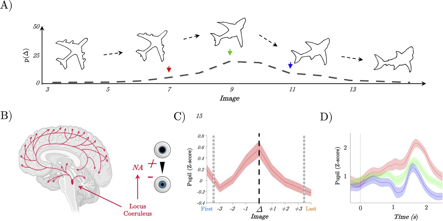
Pupil diameter tracks perceptual change.
(A) Example trial showing the continuous change from a stable image (plane) into a shark; Lower: the probability of detecting a switch (Δ) as a function of Image – most switches occur around the mid-point, but not exclusively so, leading to our prediction of heightened locus coeruleus activity at the switch point. (B) Representation of the locus coeruleus (red), its diffuse projections to the whole-brain network and its link to pupil dilation. (C) Pupil diameter group average evoked response time locked to the perceptual change (dark line, t=0). We observed an increase of the pupillary response that peaked at the perceptual change. (D) Group average of evoked pupillary responses to image switches – red represents the faster response when the switch occurs at image 6; green indicates a medium response with the switch at image 8; and blue denotes the slowest response with the switch at image 10.
Figure 2 with 2 supplements
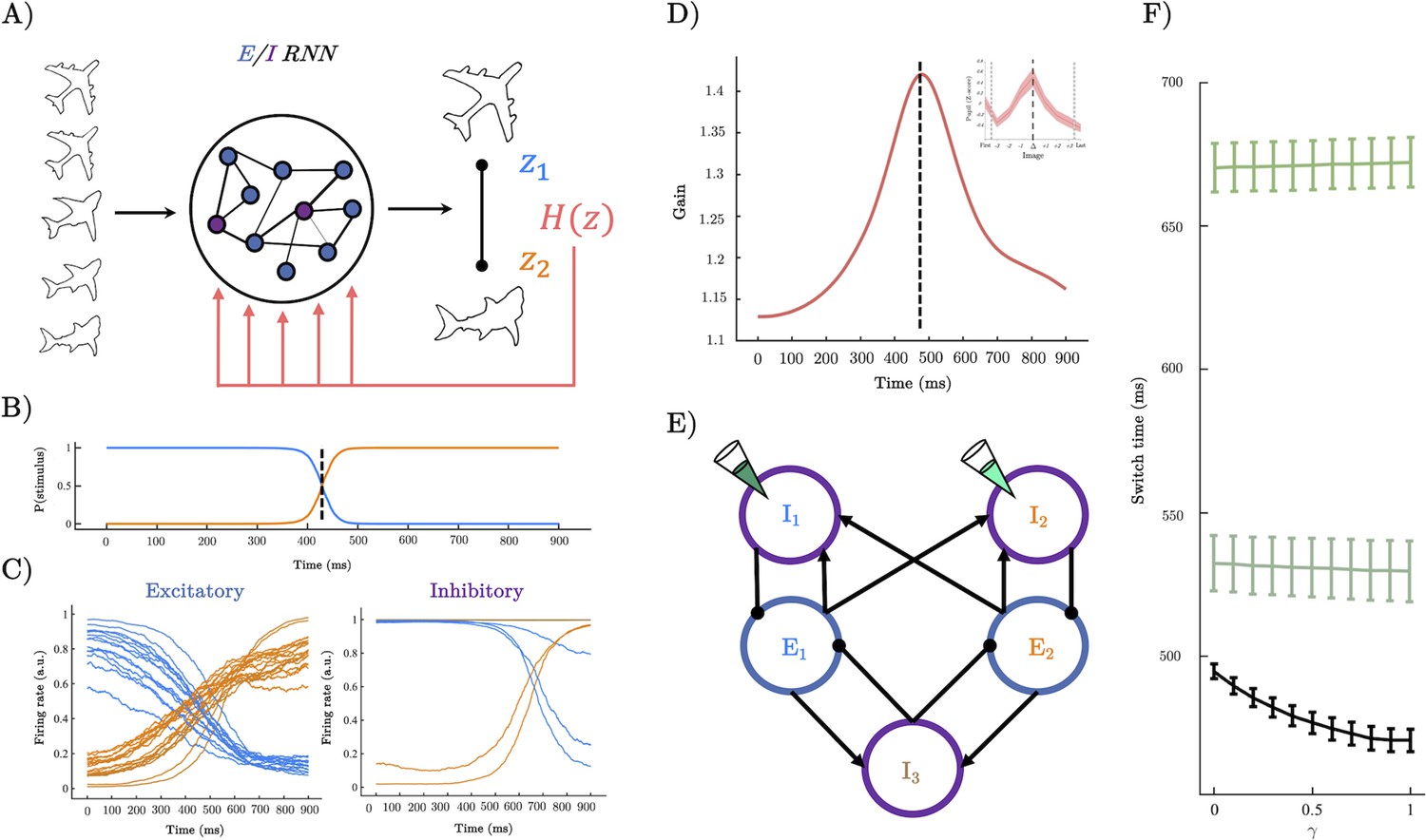
A recurrent neural network (RNN) model of perceptual switching.
(A) We trained a continuous time E/I RNN to categorise linearly changing inputs representing two discrete categories (e.g. output z1 and output z2). (B) Softmax of network outputs on example trial with , dotted line shows the timing of the perceptual switch. (C) Following training, the firing rate of the excitatory units was clearly separated into two stimulus-selective clusters – those that responded maximally to u1 (blue) and those that respond maximally to u2 (orange). Inhibitory units demonstrated a similar modular clustering but were sorted by the selectivity of the excitatory units they inhibited. (D) Dynamics of gain on example trial with which peaks close to the perceptual switch (inset shows similarity to pupil diameter). (E) Simplified network structure implied by selectivity analysis. Excitatory units (blue) form two stimulus-selective modules. Each excitatory cluster is inhibited by a cluster of inhibitory units and a third non-selective inhibitory population. Pipette shows lesion targets. (F) Switch time as a function of magnitude (i.e. magnitude of uncertainty forcing). Lower black line shows a speeding effect of heightened (and therefore heightened gain at the perceptual switch). Teal lines show switch time for lesions to the inhibitory population targeting the initially dominant population (dark teal upper), and lesions to the inhibitory population selective for the stimulus the input is morphing into (light teal middle).
Figure 2—figure supplement 1

Switch time as a function of gain for the network simulated with static (i.e. constant) gain.
Figure 2—figure supplement 2
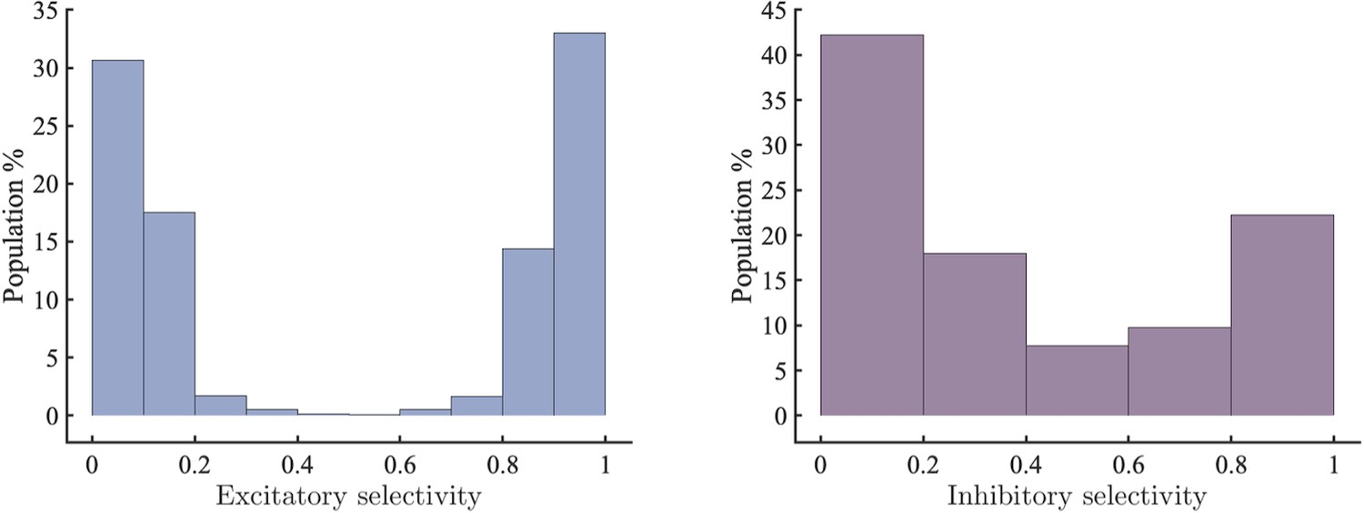
Left selectivity of excitatory units (0: completely selective for , 1: completely selective for ).
Right selectivity of inhibitory units sorted by the degree to which they inhibit excitatory units with selectivity >0.5 or <0.5.
Figure 3 with 1 supplement
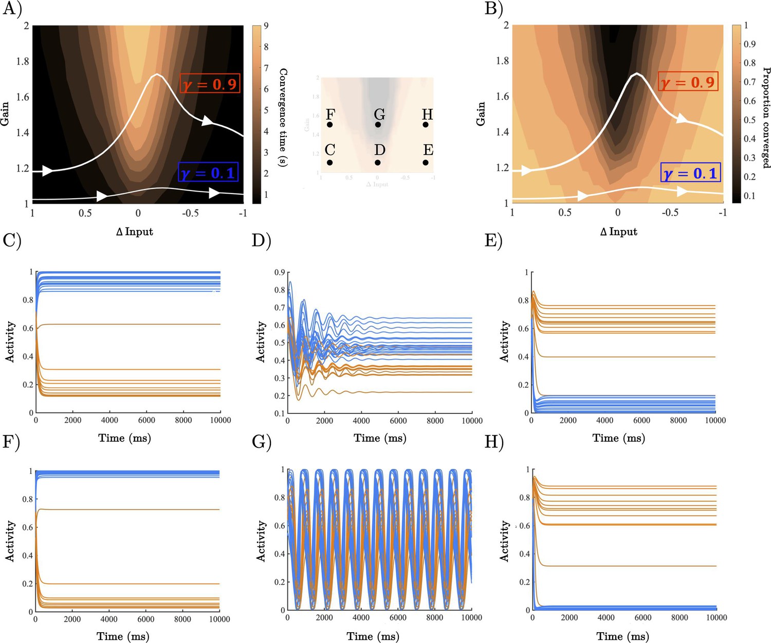
Analysis of recurrent neural network (RNN) dynamical regime.
(A) Contour map of convergence time across the full gain by Δinput parameter space averaged across 100 initialisations with random initial conditions. Example parameter trajectories shown in white for high and low γ trials. (B) Contour map of convergence proportion across the full parameter space. (C–E) Example dynamics with gain = 1.1 and Δinput ≈ [1, 0],[. 5, .5], and [0,1] r, respectively. (F–H) Example dynamics with gain = 1.5 and Δinput ≈ [1, 0],[. 5, .5], and[0,1] , respectively.
Figure 3—figure supplement 1

Example network dynamics initialised with parameter values well inside the oscillatory regime (, gain = 1.5) with initial conditions determined by the selectivity of each unit.
Excitatory units selective for , and the associated inhibitory units, were fully activated. Excitatory units selective for (and the associated inhibitory units) were initially silenced. Example network conforms with our prediction displaying an out-of-phase oscillation where the initially dominant population is rapidly silenced and the competing population is boosted after a brief delay.
Figure 4 with 1 supplement
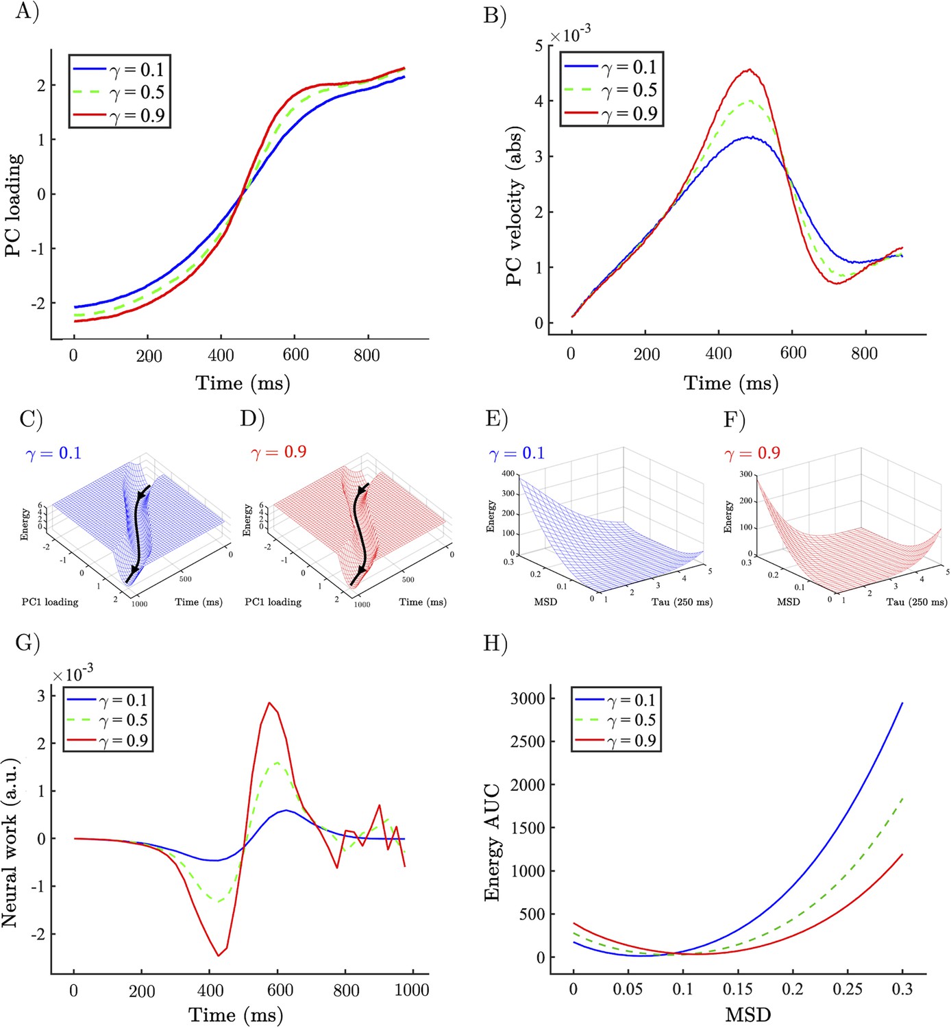
Allocentric and egocentric energy landscape dynamics underlying the perceptual speeding effect of heightened gain.
(A) Example network trajectory projected onto PC1 and averaged across trials for low (0.1; solid blue), medium (0.5; dotted green), and high (0.9; solid red) for the condition. (B) (abs) Velocity of PC1 trajectories across low (0.1), medium (0.5), and high (0.9) . (C, D) Allocentric landscapes for low (0.1; blue) and high (0.9; red) conditions. Trial-averaged PC1 trajectory shown in black. For purposes of visualisation energy, values > 6 are set to a constant value. (E, F) Egocentric landscapes for low (0.1; blue) and high (0.9; red) conditions. (G) (Allocentric) neural work for low (0.1), medium (0.5), and high (0.9) averaged across networks and conditions. (H) Egocentric AUC for low (0.1), medium (0.5), and high (0.9) averaged across networks and conditions. Note that the time series represent simulations from a model with low noise, and hence did not require error bars.
Figure 4—figure supplement 1
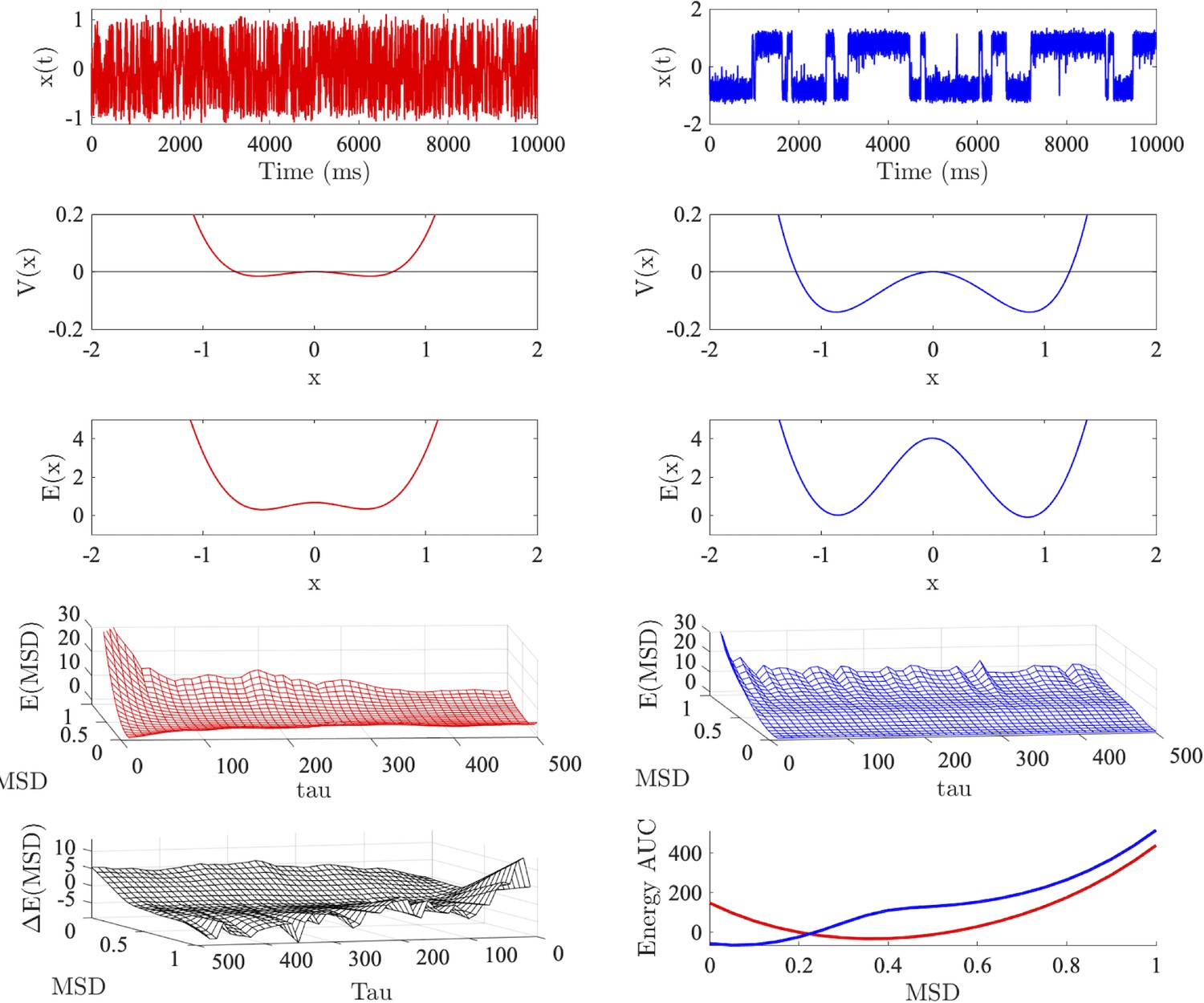
Energy landscape analyses.
Top row: time series generated from a (super critical) pitchfork bifurcation with (red left) and (blue right), respectively, simulated in the presence of noise ().
Second row: the potential for each dynamical system. Third row: allocentric landscape recovers the shape of the (analytic) potential with the depth and minima of each energy well scaling with . Fourth row: shallow and deep potentials are associated with high and low energy for large MSD values (respectively). Fifth row left: egocentric landscape with minus egocentric landscape with . X and Y axes have been reversed for visual interpretability. Fifth row right: energy under the curve for each landscape obtained by summing over time.
Figure 5 with 1 supplement
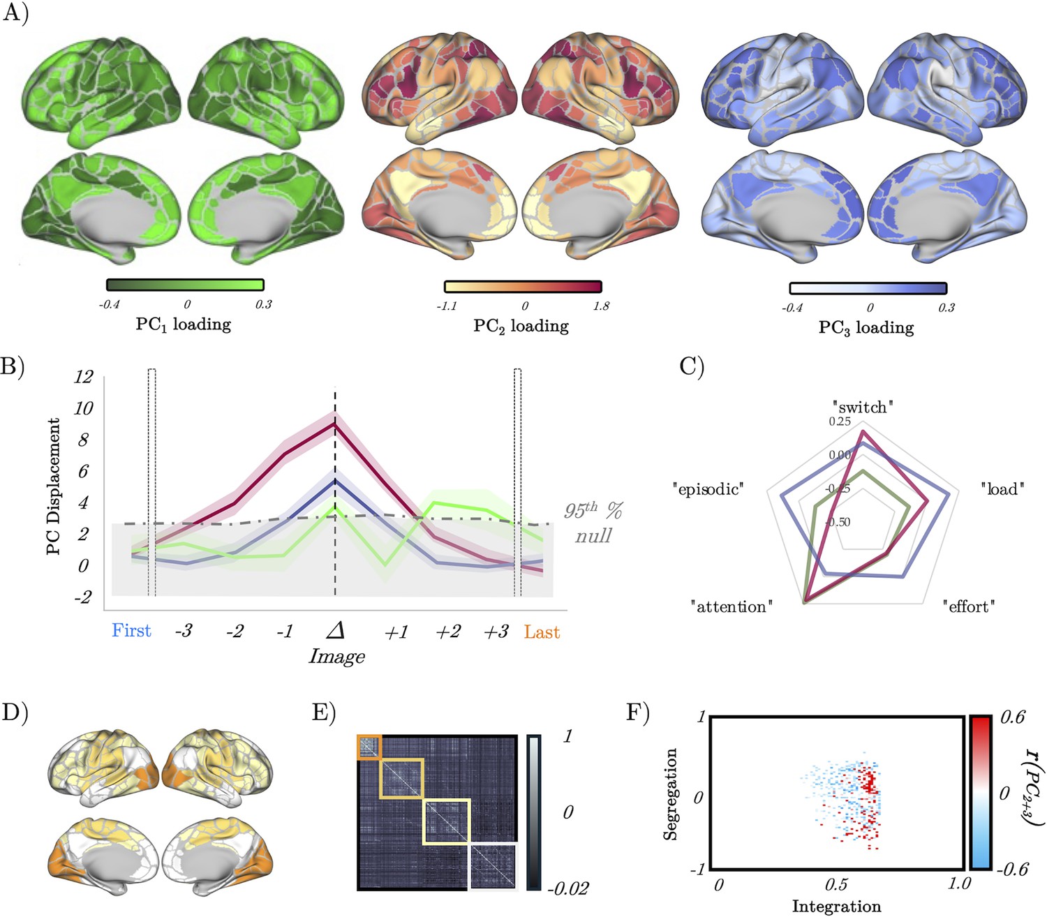
Low-dimensional switch-related dynamics and connectivity.
(A) Spatial loadings of PC1 (green), PC2 (red), and PC3 (blue). (B) Mean absolute β loading (solid lines) and group standard error (shaded) of PC1 (green), PC2 (red), and PC3 (blue), organised around the image switch point (Δ) – the dotted grey lines show the 95th percentile of the null distribution of a block-resampling permutation. (C) Radar plot showing the partial correlations of PC1 (green), PC2 (red), and PC3 (blue). (D) Evoked brain activity of PC2 + PC3 during the perceptual switch. (E) Group averaged functional connectivity and module assignments using a Louvain analysis – three clusters were observed. (F) Pearson’s correlation between the sum of PC2 and PC3 (per subject) and a joint-histogram comparing Integration (participation coefficient) and segregation (module-degree Z-score); p<0.05 following permutation testing.
Figure 5—figure supplement 1

Energy landscape analyses.
(A) Pearson’s correlation between each PCs and the evoked brain activity at the perceptual switch (β values), dashed line at PC2. (B) Pearson’s correlation between the inverted brain maps using βPC (PC(1-i) × βPC(1-i)). Dashed line shows that the correlation gets to 94% using the first three PCs (Pearson’s r=0.94, p<0.001).
Figure 6
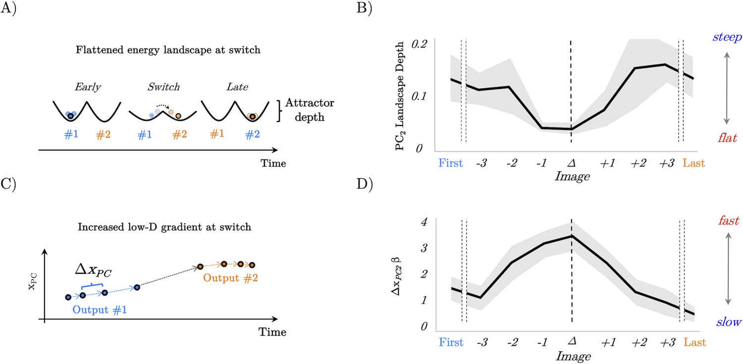
Confirmation of model predictions in whole-brain BOLD data.
(A) analysis of the recurrent neural network (RNN) also predicted that the energy landscape dictating the likelihood of state transitions should be flat (i.e. have a small attractor depth) at the switch point. (B) The energy landscape was demonstratively flatter (quantified as surprisal over brain activity displacement) at the switch point. (C) By interrogating the low-dimensional trajectories in the RNN, we predicted that there should be a peak in the gradient of the loadings in principal component space at the switch point between output #1 and output #2. (D) The gradient (ΔxPC) of the β loading of PC2 as a function of the switch point.
Additional files
Download links
A two-part list of links to download the article, or parts of the article, in various formats.
Downloads (link to download the article as PDF)
Open citations (links to open the citations from this article in various online reference manager services)
Cite this article (links to download the citations from this article in formats compatible with various reference manager tools)
Evidence from pupillometry, fMRI, and RNN modelling shows that gain neuromodulation mediates task-relevant perceptual switches
eLife 13:RP93191.
https://doi.org/10.7554/eLife.93191.4


