Volumetric trans-scale imaging of massive quantity of heterogeneous cell populations in centimeter-wide tissue and embryo
- Transdimensional Life Imaging Division, Institute for Open and Transdisciplinary Research, Initiatives, Osaka University, Osaka University, Japan
- Department of Biomolecular Science and Engineering, SANKEN, Osaka University, Japan
- SIGMAKOKI CO LTD, Midori, Sumida-ku, Japan
- Department of Anatomy and Cell Biology, Graduate School of Medical Sciences, Kyushu University, Japan
- Laboratory of Molecular Neuropharmacology, Graduate School of Pharmaceutical Sciences, Osaka University, Japan
- Laboratory for Developmental Dynamics, RIKEN Center for Biosystems Dynamics Research, Japan
- Research Institute for Electronic Science, Hokkaido University, Japan
Figures
Figure 1
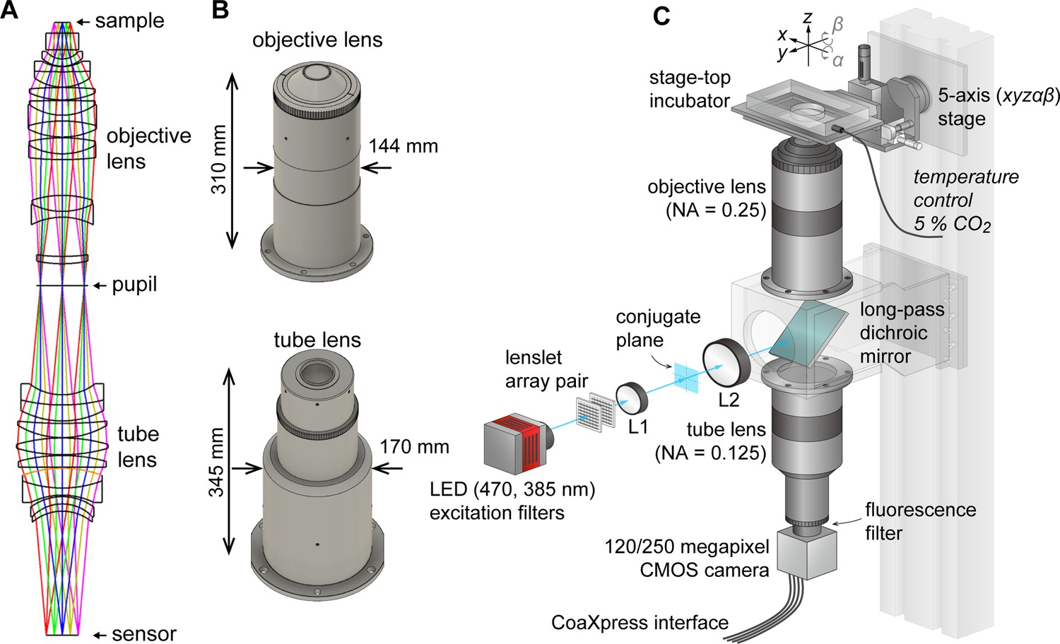
AMATERAS-2, a centimeter-FOV cell-imaging system.
(A) Schematics of the design of the objective and tube lenses for AMATERAS-2. (B) Appearance of the objective and tube lenses with the width and length. (C) Diagram of the wide-field fluorescence imaging system, AMATERAS-2w, using the two lenses in (A–B). See Materials and methods for detail.
Figure 2 with 1 supplement
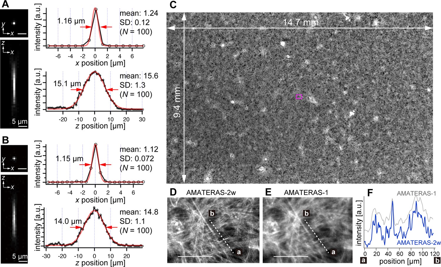
Optical performance of AMATERAS-2w.
(A, B) Experimentally obtained PSF of green fluorescent beads with a 0.2 µm diameter in the xy and xz planes, captured using CMOS cameras with (A) 120 megapixels (pixel size=2.2 µm) and (B) 250 megapixels (pixel size=1.5 µm). The representative line profiles in the x and z directions on the beads are shown (black lines with circular markers) along with Gaussian fit curves (red lines) and FWHMs, and the mean and standard deviation (SD) calculated for 100 beads are described beside each profile. (C) Fluorescence image of a cardiomyocyte sheet in the entire FOV. (D) Digitally magnified view of the area indicated by a magenta square at the center of (C); scale bar, 100 µm. (E) Same area as (D) but observed by AMATERAS-1 for comparison. (F) Line profiles of the lines in (D) and (E) for comparison of spatial resolution.
Figure 2—figure supplement 1
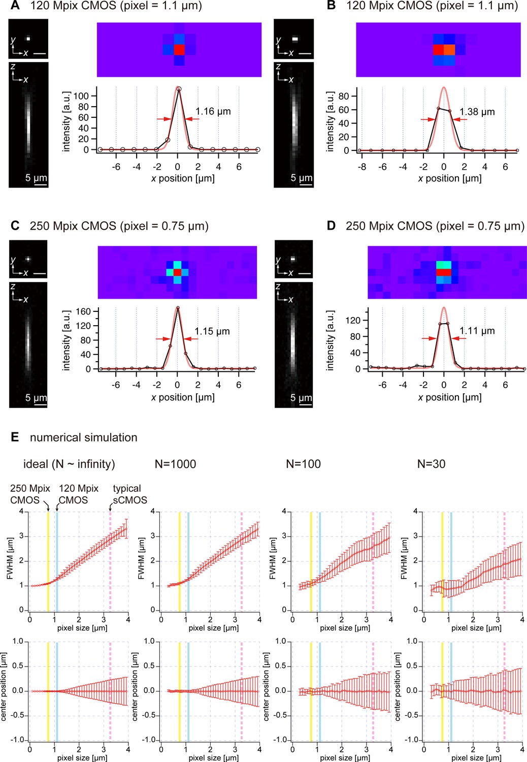
Uncertainty in spatial resolution and position owing to undersampling.
(A, B) Two cases of images of fluorescent beads (diameter, 0.2 µm) captured using the 120-megapixel camera. (C, D) Two cases of images of fluorescent beads (diameter, 0.2 µm) captured using the 250-megapixel camera. (E) Dependence of FWHM and center position on pixel size, as revealed by a numerical simulation. The number of photon (N) is varied from N~infinity, 1000, 100, and 30.
Figure 3 with 2 supplements
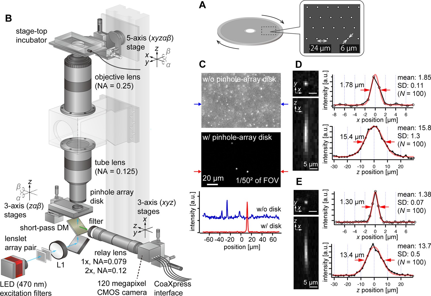
AMATERAS-2c, a multipoint confocal imaging system for 3D volume imaging.
(A) Design of our pinhole-array disk. (B) Schematic of the optical configuration using the pinhole-array disk. (C) Effect of background light rejection by the presence of the pinhole-array disk in a 292×202 µm2 area at the FOV center corresponding to 1/502 of the entire FOV. (D, E) Experimentally obtained PSF of green fluorescent beads with a diameter of 0.5 µm in the xy and xz planes, captured using relay lens with (D) ×1 magnification (NA=0.079) and (E) ×2 magnification (NA=0.12). The representative line profiles in the x and z directions on the beads are also shown (black lines with circular markers) along with Gaussian fit curves (red lines) and FWHMs, and the mean and standard deviation (SD) calculated for 100 beads are described beside each profile.
Figure 3—figure supplement 1
Schematic configuration of the confocal system and the effect of the pinhole size.
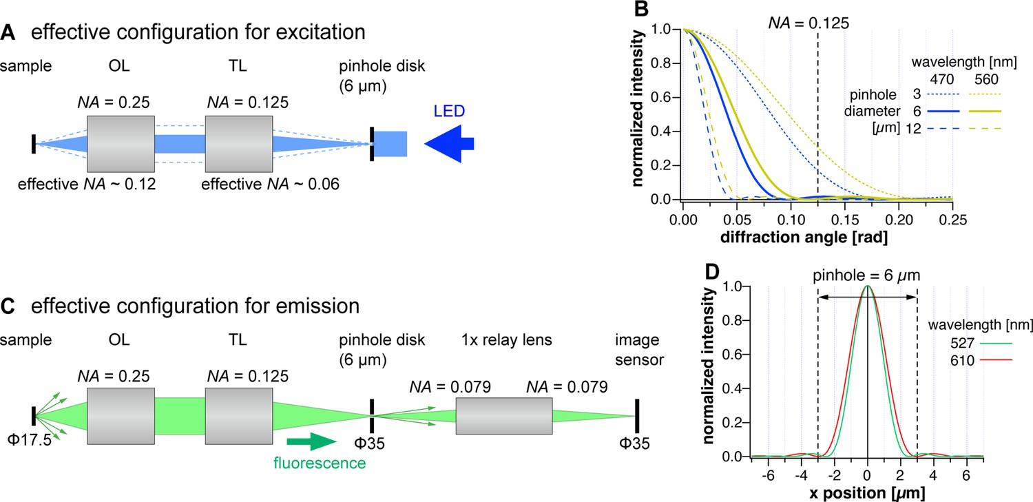
(A) Effective configuration for excitation in the confocal imaging system, AMATERAS-2c. OL and TL denote objective lens and tube lens, respectively. (B) Diffraction pattern by a pinhole with various conditions (wavelength and pinhole diameter), calculated by Equation 1. The intensity of diffracted light is plotted as a function of diffraction angle. The diffraction angle equivalent to the NA of the tube lens is represented by the dotted line. (C) Effective configuration for emission in AMATERAS-2c. (D) Intensity distribution of focused light spot by tube lens with 0.125 NA at the two fluorescence wavelengths (527 and 610 nm). The size of the 6 µm pinhole is indicated by the dashed lines.
Figure 3—figure supplement 2
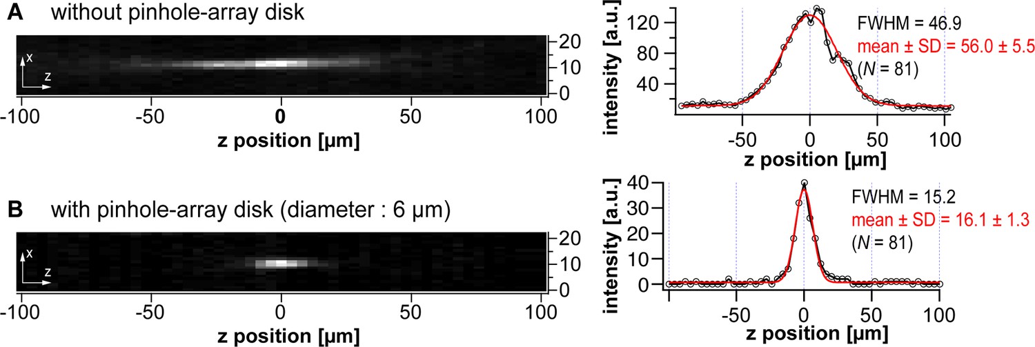
Evaluation of the optical sectioning effect by the confocal system.
(A–B) Point-spread functions measured in the absence (A) and presence (B) of the pinhole-array disk (diameter: 6 µm). The optical configuration for this experiment employed the ×1 relay lens, the same as used in Figure 3D in the main text (total magnification: ×2). Left panels show xz planes centering at a single fluorescent bead. Right panels show the line profiles in the z direction across the bead positions in the left panels. The FWHMs are noted alongside the line profiles. The statistical values of 81 peaks are also shown as well.
Figure 4 with 4 supplements
Volumetric imaging with computational sectioning.
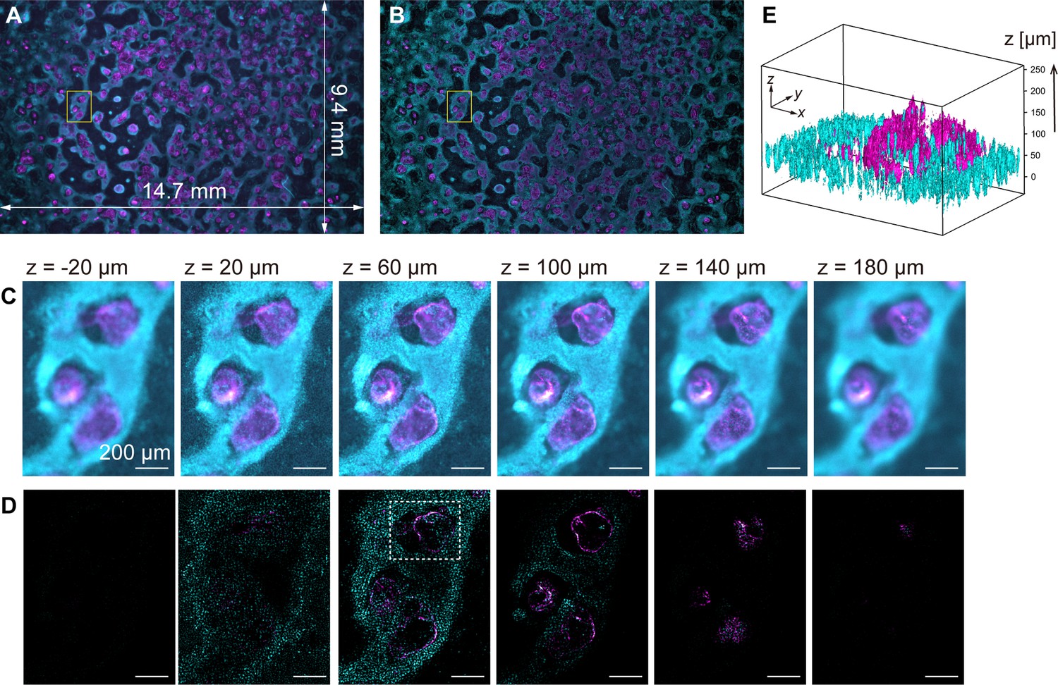
(A, B) Two-color images of the cavity chamber structure of a myocardial organoid (A) before and (B) after computational sectioning. Both (A) and (B) are MIP images of the z-stack data, captured using the 250-megapixel CMOS camera; here, magenta and cyan represent the distribution of immunostained cardiac troponin T and Hoechst-labeled nuclei, respectively. (C, D) Six z-layers with a difference of 40 µm in the yellow square region indicated in (A, B); scale bars, 200 µm. (E) Three-dimensional isosurface representation in the dashed square region indicated in (D).
Figure 4—figure supplement 1
Performance of computational sectioning with varied cutoff frequency.
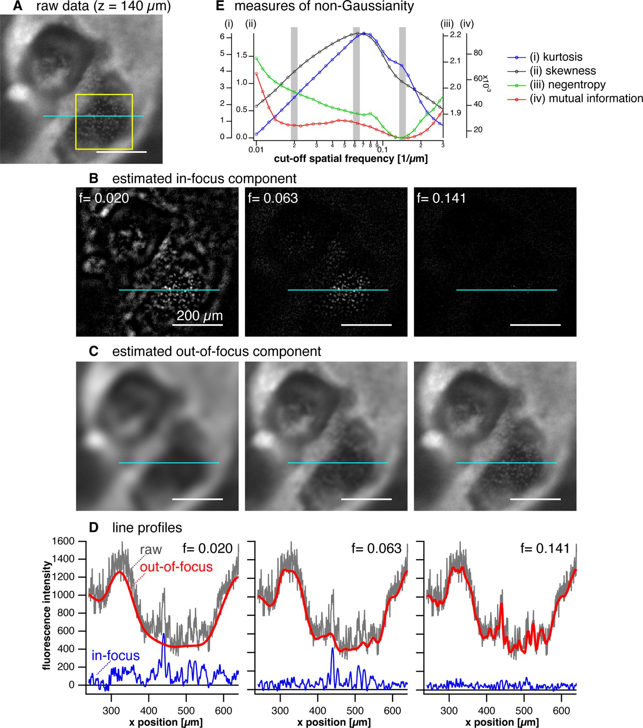
(A) A raw image data, a local area of a z-layer (z = 140 µm) in a z-stack data of a dome structure of a myocardial organoid, which is shown in Figure 4 in the main text. (B–C) Estimated in-focus images (B) and out-of-focus images (C) for three different cutoff frequencies, Fc=0.020, 0.063, and 0.141. Scale bar (white line): 200 µm. (D) Line profiles of intensity on the light-blue lines drawn in A, B, and C. (E) Four types of statistical measures for non-Gaussianity calculated as a function of cutoff frequency of the low-pass filter. The values were calculated for the in-focus image in the yellow square region. The three frequencies used for the image examples (B–D) are indicated by gray bars. See Appendix File – Note 2 for more detail.
Figure 4—figure supplement 2
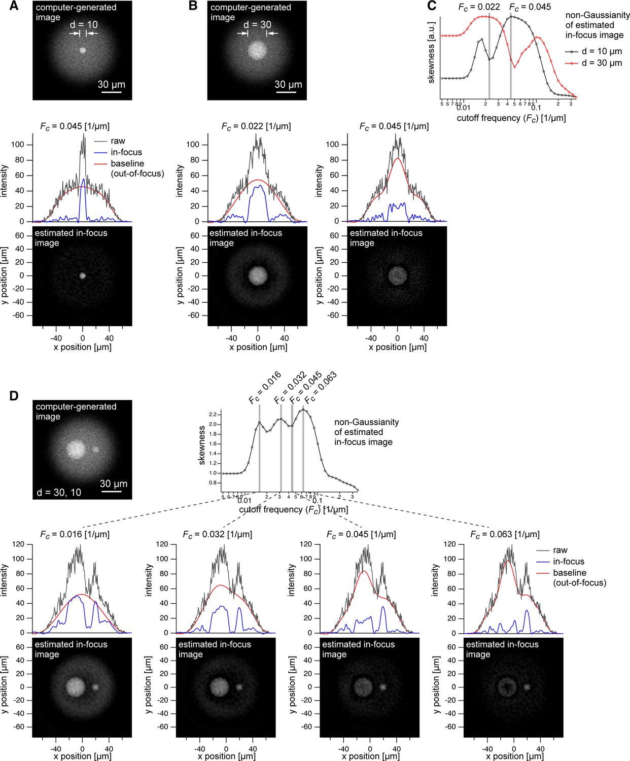
Dependence of baseline estimation performance on object size.
(A–B) Top: Computer-generated fluorescence image of superposition of a 10 µm sphere and a 30 µm sphere (object) and a 50 µm sphere placed 100 µm deep (background). Bottom: Estimated in-focus image at the cutoff frequency of 0.045 and 0.022 (only in B). Line profiles of the raw, estimated in-focus and out-of-focus images are shown on the images. (C) Frequency dependence of the non-Gaussianity (skewness) of in-focus image for the 10 µm and 30 µm spheres. (D) Top: Computer-generated fluorescence image of superposition of a 30 µm sphere and a 10 µm sphere (object) and a 50 µm sphere placed 100 µm deep (background). Bottom: Estimated in-focus image at four cutoff frequencies (0.016, 0.032, 0.045, and 0.063) shown with line profiles of raw, in-focus and out-of-focus images. See Appendix File – Note 2 for more detail.
Figure 4—video 1
A z-stack of a cavity chamber structure of myocardial organoid (left) without and (right) with the computational sectioning, corresponding to Figure 4C and D, respectively.
The z-position is swept with a step of 4 µm in 56 layers. Magenta and cyan colors represent the distribution of immunostained cardiac troponin T and Hoechst-labeled nuclei, respectively.
Figure 4—video 2
A 3D isosurface representation of a dome structure of cavity chamber with varying the view angle.
The cropped region is indicated by a dashed square in Figure 4D.
Figure 5 with 2 supplements
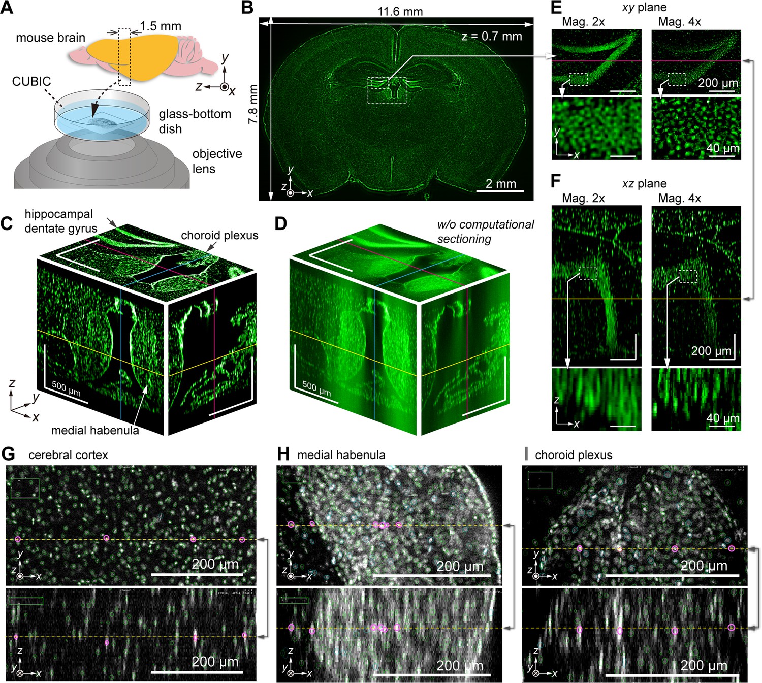
Volumetric imaging of a mouse brain section obtained by AMATERAS-2c.
(A) Schematic of a mouse brain showing the placement of the brain sample in the inverted configuration. (B) Schematic of a single z-layer in the coronal plane with size of the effective area covering the entire brain section. (C) Fluorescence images of three orthogonal cross sections of the dotted square indicated in (B); here, the yellow, cyan, and magenta lines represent the z-, x-, and y-positions of the cross sections, respectively. (D) Cross-sectional images of raw data in the same region as (C), where the computational sectioning is not applied. (E, F) Magnified images of the hippocampal region (dashed square in (B)) in the (E) xy-plane and (F) xz-plane. For comparison, images obtained with ×2 (left) and ×4 (right) magnification systems are shown together. Note that the 3D regions observed at different magnifications do not perfectly match owing to the difficulty in optical alignment. (G–I) Cell detection by ELEPHANT in three brain regions, the cerebral cortex (G), medial habenula (H), and choroid plexus (I), where pairs of intersecting xy- and xz-planes are arranged vertically. The detected cells within each plane are marked with green and cyan ovals, and the straight line shared by the two planes is represented by a yellow dashed line, with certain cells along this line highlighted by magenta ovals. The xy-planes overlay the oval markers within a range of ±25 µm above and below the displayed planes, while the xz-planes show only oval markers on the planes.
Figure 5—video 1
A z-stack of the mouse brain section shown in the full coronal plain region (Figure 5B).
The z-position is swept with a step of 4 µm in 378 layers.
Figure 5—video 2
A z-stack of the mouse brain section shown in the local volume corresponding to Figure 5C.
The z-position is swept with a step of 4 µm in 378 layers.
Figure 6 with 5 supplements
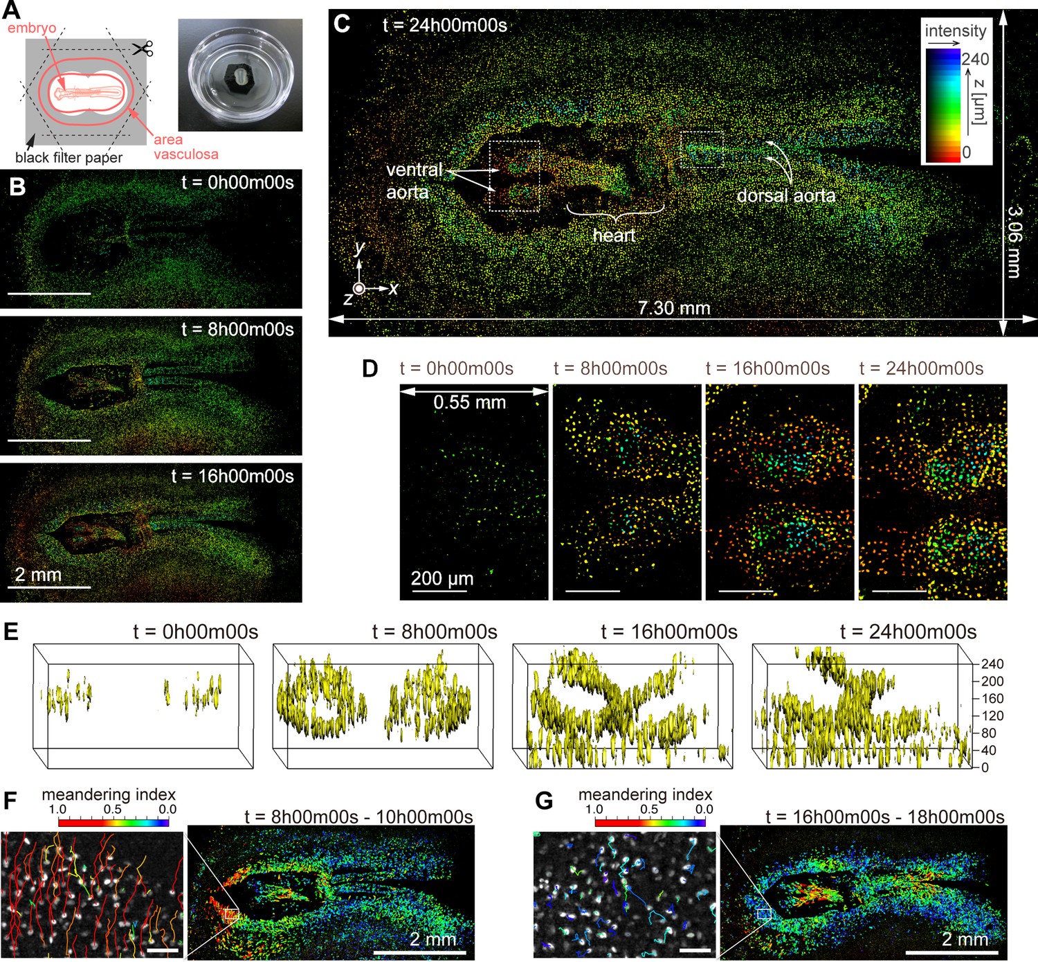
Dynamics of vascular endothelial cells in quail embryo captured by time-lapse observation.
(A) Schematic showing how the specimen is mounted (left) and a photograph of a specimen placed in a glass-bottom dish. (B) Representative images obtained at t=0 hr, 8 hr, and 16 hr; scale bars, 2 mm. (C) Enlarged view of the image corresponding at t=24 hr; the pseudo-colors represent the z-position of the cells and fluorescence intensity by their hue and brightness, respectively. (D) Magnified views of the anterior side of ventral aortae (left dashed square in (C)) at the four time-points with intervals of 8 hr; scale bars, 200 µm. (E) Three-dimensional isosurface representation of the dorsal aorta region (right dashed square in (C)) viewed from the left side. (F), (G) Cell position trajectories and spatial mapping of features related to the cell dynamics in the two time-regions of (F) t=8–10 hr and (G) t=16–18 hr. Left panels show enlarged views in the white square regions (292×202 µm2) indicated in the right panels. In both the panels, the rainbow-colored trajectories of the cell movement are overlaid on the grayscale MIP images at the first frame in the time regions (F: t=8 hr, G: t=16 hr). The scale bars are 50 µm. The rainbow color table represents the meandering index of the cell movement in the two time-regions.
Figure 6—figure supplement 1
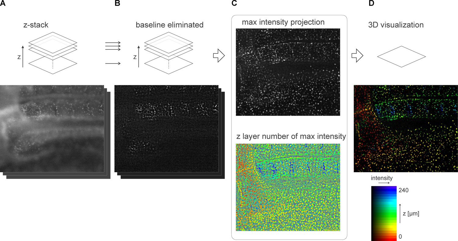
Computational processing and 3D visualization of the z-stack data of quail embryo.
(A) Raw image data. (B) In-focus component obtained by computational sectioning to eliminate the baseline component (out-of-focus component). (C) Images of projected max intensity and the z-layer number where maximum intensity is found, which are calculated from a set of z-stack. (D) Visualization of the 3D data using the HSB color table.
Figure 6—video 1
Time lapse video of the quail development in: (6) the entire body region, (7) ventral aorta region, and (8) dorsal aorta region.
The time interval is 7.5 min in 25 hr (200 time points). The rainbow color of cells denotes the z-position based on the color scale shown in Figure 6C.
Figure 6—video 2
Time lapse video of the quail development in: (6) the entire body region, (7) ventral aorta region, and (8) dorsal aorta region.
The time interval is 7.5 min in 25 hr (200 time points). The rainbow color of cells denotes the z-position based on the color scale shown in Figure 6C.
Figure 6—video 3
Time lapse video of the quail development in: (6) the entire body region, (7) ventral aorta region, and (8) dorsal aorta region.
The time interval is 7.5 min in 25 hr (200 time points). The rainbow color of cells denotes the z-position based on the color scale shown in Figure 6C.
Figure 6—video 4
Time lapse video of the dorsal aorta region (Figure 6E) in the 3D isosurface representation.
Videos
Video 1
A z-stack of the mouse brain section shown in the local volume in the cortex region.
Cells detected by ELEPHANT are indicated by green oval markers. The z-position is swept with a step of 4 µm in 50 layers (200 µm) from the surface of the brain section.
Tables
Key resources table
| Reagent type (species) or resource | Designation | Source or reference | Identifiers | Additional information |
|---|---|---|---|---|
| Genetic reagent (coturnix japonica) | tie1:H2B-eYFP | Sato et al., PLoS One. 5, e12674 (2010). | ||
| Strain, strain background (mouse) | C57BL/6JJmsSlc | Japan SLC,Inc. | RRID:MGI:5488963 | |
| Cell line (Homo sapiens) | iPS cell | Riken Cell Bank Takahashi et al., Cell 131, 861–872 (2007). | 201B7 RRID:CVCL_A324 | |
| Antibody | rabbit IgG anti-cTnT (polyclonal) | Bioss | Cat#:bs-10648R | 1:200 |
| Antibody | alexa488 conjugated goat IgG anti-rabbit IgG (polyclonal) | Abcam | Cat#:Ab150077; RRID:AB_2630356 | 1:500 |
| Other (culture medium) | CDM3 | Burridge, et al., Nat. Methods. 11, 855–860 (2014) | used for initiation of iPSC differentiation | |
| Other (culture medium) | StemFit | Ajinomoto | Cat#:AK02N | used for iPSC culture |
| Other (dish coating peptide) | iMatrix-511 | Matrixome | Cat#:89292 | used to coat a dish for iPSC culture |
| Other (cell detachment reagent) | TrypLE Select | Thermo Fisher Scientific, | Cat#:A1285901 | used to dissociate iPSCs |
| Chemical compound | Y-27632 | Fujifilm Wako | Cat#:030–24021 | |
| Chemical compound | CHIR99021 | Fujifilm Wako | CAS: 252917-06-9;Cat#:038–23101 | |
| Chemical compound | IWP-2 | Fujifilm Wako | CAS: 686770-61-6;Cat#:034–24301 | |
| Chemical compound | Medetomidine | Nippon Zenyaku Kogyo | CAS:86347-14-0 | |
| Chemical compound | midazolam | Sandoz Pharma | CAS:59467-70-8 | |
| Chemical compound | butorphanol | Meiji Seika Pharma | CAS:42408-82-2 | |
| Other (fluorescent dye) | Rhodamine phalloidin | Fujifilm Wako | Cat#:165–21641 | used for fluorescent labelling of actin filaments in the cardiac cell sheet |
| Other (fluorescent dye) | Hoechst33342 | Dojin | Cat#:H342 | used for fluorescent labelling of nuclei of cardiac organoid |
| Other (fluorescent dye) | SYTOX Green | Thermo Fisher Scientific | Cat#:S7020 | used for fluorescent labelling of nuclei in the mouse brain section |
| Other (tissue-clearing reagent) | CUBIC-L | Tokyo Chemical Industry | Cat#:T3740 | used for tissue clearing of the mouse brain section |
| Other (tissue-clearing reagent) | CUBIC-R+(M) | Tokyo Chemical Industry | Cat#:T3741 | used for tissue clearing of the mouse brain section |
| Software | ELEPHANT | Sugawara et al., 2022; Sugawara, 2024 | Server: v0.5.7i, Client: v0.5.0 | https://github.com/elephant-track |
Additional files
Download links
A two-part list of links to download the article, or parts of the article, in various formats.
Downloads (link to download the article as PDF)
Open citations (links to open the citations from this article in various online reference manager services)
Cite this article (links to download the citations from this article in formats compatible with various reference manager tools)
Volumetric trans-scale imaging of massive quantity of heterogeneous cell populations in centimeter-wide tissue and embryo
eLife 13:RP93633.
https://doi.org/10.7554/eLife.93633.3


