Pan-cortical 2-photon mesoscopic imaging and neurobehavioral alignment in awake, behaving mice
- Institute of Neuroscience, University of Oregon, United States
- Department of Biology, University of Oregon, United States
Figures
Figure 1 with 2 supplements
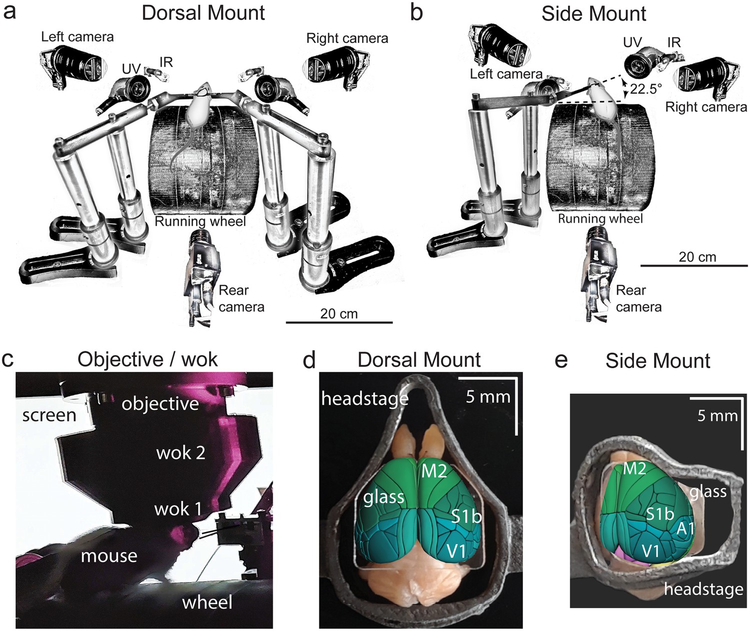
Technical adaptations for dual-mount in vivo pan-cortical imaging with the Thorlabs 2p-RAM mesoscope.
(a) Mesoscope behavioral apparatus for the dorsal mount preparation. Mouse is mounted upright on a running wheel with headpost fixed to dual adjustable support arms mounted on vertical posts (1” diameter). Behavior cameras are fixed at front-left, front-right, and center-posterior, with ultraviolet and infrared light-emitting diodes aligned with goose-neck supports parallel to right and left cameras. (b) Mesoscope behavioral apparatus for side mount preparation. Same as in (a), except that the mouse is rotated 22.5 degrees to its left so that the objective lens (at angle 0) is orthogonal to the center-of-mass of the preparation across the right cortical hemisphere. The objective can rotate +/-20 degrees medio-laterally, if needed, to optimize imaging of any portion of the cortex under the cranial window. The right behavior camera is positioned more posterior and lower than in (a), to allow for imaging of the eye under the acute angle formed with the horizontal light shield, shown in (c). (c) Mouse running on wheel with side mount preparation receiving visual stimulation from an LED screen positioned on the left side, with linear motor-positioned dual lick-spouts in place and 3D printed vertical light shield (wok 2) attached to rim of flat shield (wok 1) to block extraneous light from entering the objective. (d) Overhead view of dorsal mount preparation with 3D printed titanium headpost, custom cranial window, and Allen CCF aligned to paraformaldehyde-fixed mouse brain. Motor region = light green, somatosensory = dark green, visual = dark blue, retrosplenial = light blue. Olfactory bulbs (anterior) at top, cerebellum (posterior) at bottom of image. Note ridge along perimeter of headpost for fitted horizontal light shield (wok 1) attachment. (e) Rotated dorsal view (22.5 degrees right) of side mount preparation with 3D printed titanium headpost, custom cranial window, and Allen CCF aligned to paraformaldehyde-fixed mouse brain. Auditory region shown in light blue, ventral and anterior to visual areas, and ventral and posterior to somatosensory areas (right side of image is lateral/ventral, and left side of headpost perimeter is medial/dorsal). Other regions shown with the same color scheme as in (d). UV = ultraviolet, IR = infrared, M2 = secondary motor cortex, S1b = primary somatosensory barrel cortex, V1 = primary visual cortex, A1 = primary auditory cortex.
Figure 1—figure supplement 1
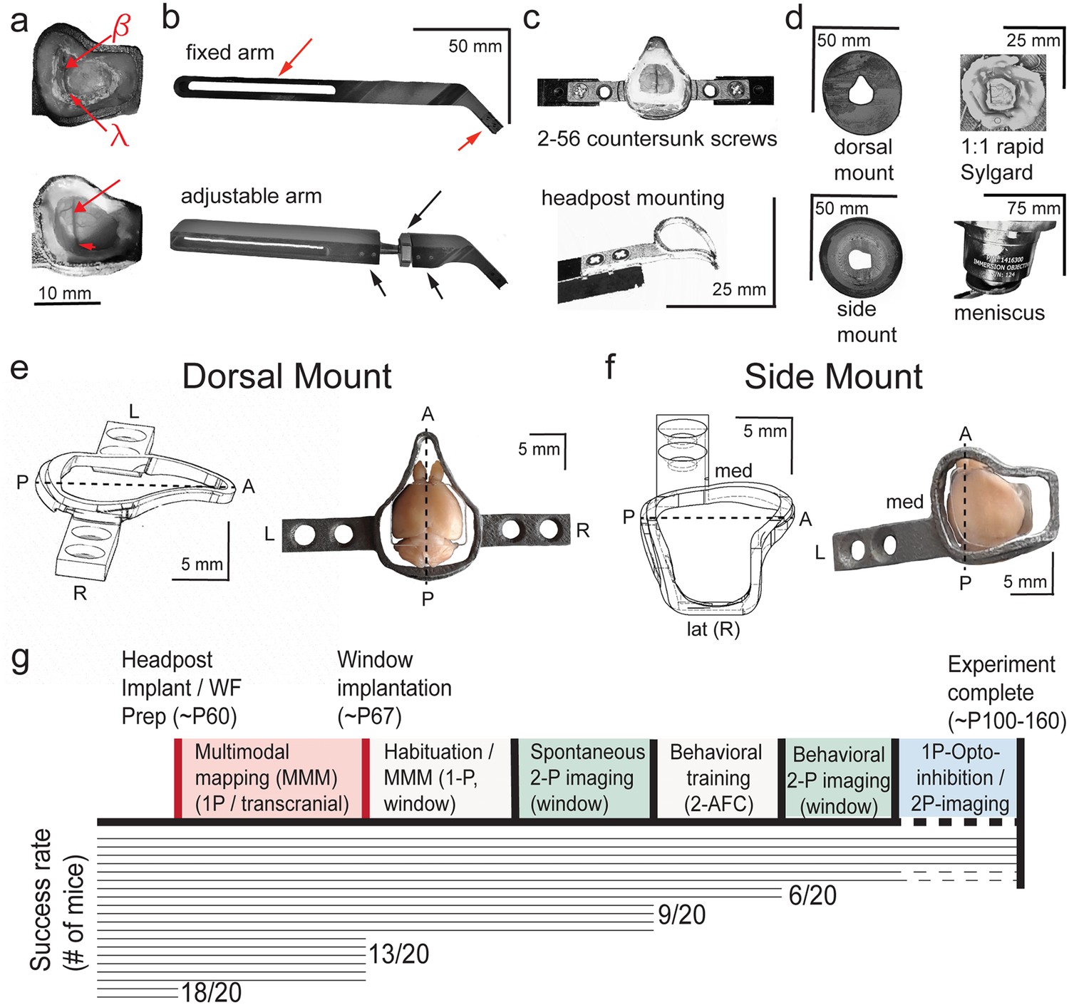
Detailed technical adaptations for dual-mount in vivo pan-cortical imaging with 2p-RAM mesoscope.
(a) Photographs of widefield through-skull (top) and 2-photon cranial window (bottom) states of side mount preparation. Bregma (β) and lambda (λ) skull landmarks used in multimodal mapping alignment to common coordinate framework (CCF) map are indicated (top), along with their corresponding positions relative to cortical blood vessels visible through cranial window (bottom). Note that all visible tissue inside the perimeter of the headpost in the lower image is seen through curved, 210-µm-thick borosilicate Schott D263 glass. (b) Custom aluminum support arms for use with both dorsal mount and side mount preparations. Fixed arm (top) has flat proximal angle at bend near dual-screw headpost mounting slot (right red arrow), and can be mounted on a Thorlabs 1-inch diameter post mounted to a rotating ball-joint base (SL20, see Supplementary methods and materials) to achieve leftward 22.5 degree rotation for side mount (not shown). Flexible positioning on wheel is possible due to ¼”–20 bolt accepting slot that allows support posts to be positioned closer to or farther from headpost mounting slot (left red arrow). Custom adjustable arm (bottom) has rotating brass shaft attached to ball-and-socket joint with hexagonal tightening ring (top, long black arrow), stabilized by dual set screws on both ends (bottom, two short black arrows), at a bend proximal to the headpost mounting slot. This allows for rapid, fixable on-rig fine adjustment of the mounting angle in all directions, and eliminates the need for a Thorlabs rotating ball-joint base so that 1” diameter vertical posts can be used (instead of ½” diameter, which we used at first), thus enhancing overall stability for imaging. (c) Examples of headpost mounting for dorsal mount (top, with cranial window) and side mount (bottom, headpost only). Both headposts are attached with two 82 degree countersunk 2–56 thread 1 ⁄ 4 '' stainless steel screws (McMaster-Carr, see Supplementary methods and materials) and positioned in a custom machined slot within the support arm for enhanced stability. The headpost arm can easily be held within the support arm slot by thumb prior to screw affixation during mounting. (d) Mounting of 3D printed light shields and application of objective to water meniscus. Flat shields (top left, bottom left) are attached with 1:1 rapid curing Sylgard (top right; 170 Fast Cure encapsulant, see Supplementary methods and materials) to the perimeter of the headpost. Stable positioning during curing is enabled by attachment of dual 3-pronged lab clamps attached to left and right support arms with quick ties (not shown). Then, a tip-clipped transfer pipette is used to add deionized or Millipure water to the window, with the Sylgard acting as a dam, until the objective can be lowered far enough to raise a meniscus. Additional water can then be added from either side of the preparation under the objective. (e) Side view 3D rendering (left, from AutoDesk Inventor; L = left, R = right, A = anterior, P = posterior, center-line = dashed line) and top view photograph with cranial window placed on paraformaldehyde-fixed brain, for dorsal mount preparation. (f) Same as in (e), but for side mount preparation. (g) Cumulative success rate ‘survivorship’ diagram for dorsal and side mount preparations (note: survival rate is higher, but some preparations are not fully imageable, some mice fail to acquire the task, etc), loosely based on empirical data from mice both used to develop the preparations, those used in this study, and those used in pilot experiments for 2-alternative forced choice (2-AFC) behavior. Note that the standard full timeline involves around 100 days from headpost implantation to experiment completion. In our experience, successful cranial windows last between 100 and 150 days, or in some rare cases up to 300 days.
Figure 1—figure supplement 2
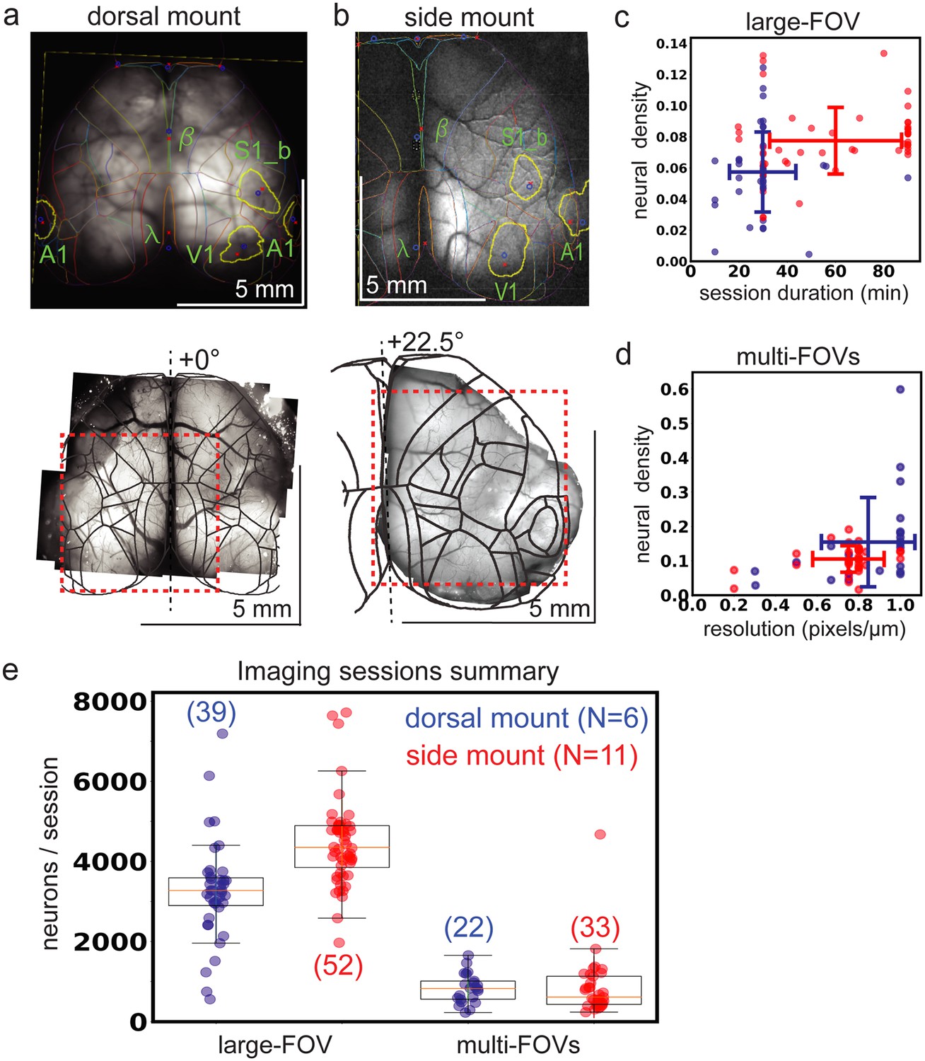
Widefield-imaging based dual-mount multimodal CCF alignment, ROI detection, and areal assignment of GCaMP6s+ excitatory neurons.
(a) Example MMM to CCF alignment for dorsal mount, shown projected onto a through-the-skull vasculature image and including skull landmarks (top). The series of user-selected points used for alignment of the widefield image onto the CCF map are shown as blue points, with corresponding red points showing the actual mapping locations used by the affine transformation. 2p-RAM pseudo-widefield vasculature montage from the same mouse, with boundaries of an example 2-photon imaging session FOV shown as a red dashed line (bottom). View angle relative to orthogonal indicated at top of dashed black line indicating mid-line. (b) Same as in (a), but for example side mount preparation. (c) Density of Suite2p-detected ROIs (density of 1 equal to one neuron per 25 x 25 µm square; total large FOV area generally 5000 x 4620 µm) for large field of view (FOV) 2-photon imaging sessions as a function of session duration for dorsal mount (blue) and side mount (red) preparations. (d) Neural density as a function of imaging resolution for 2-photon imaging sessions where multiple smaller FOVs were imaged pseudo-simultaneously. Same density calculation used as in (c), for multi-FOV sessions where the dimensions of each small FOV are generally between 660 x 660 and 1320 x 1320 µm. Here, a resolution of 0.2 pixels / µm would correspond to 5 µm per pixel resolution in both x and y dimensions (i.e. ⅕=0.2). (e) Summary statistics for all 2p imaging sessions in the current study that passed quality control for all data modalities (i.e. MMM, 2p, behavior video, etc). The number of neurons per 2p imaging session is shown for both large- (two columns at left) and small- (two columns at right) FOV sessions, split by mount type (dorsal mount in blue, side mount in red). Numbers in parentheses indicate total session counts (“S”), “N” indicates number of mice with each mount type. FOV = field of view, V1 = primary visual cortex, A1 = primary auditory cortex, S1_b = primary somatosensory barrel cortex, ß = bregma, λ = lambda.
Figure 2
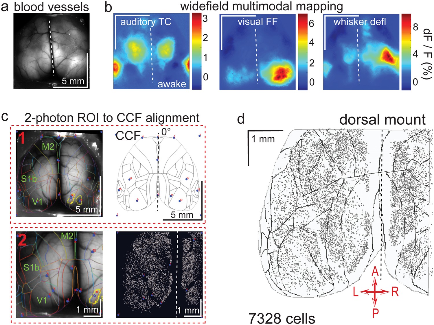
Widefield-imaging-based multimodal mapping (MMM) and CCF alignment, ROI detection, and areal assignment of GCaMP6s+ excitatory neurons for the dorsal mount preparation.
(a) Mean projection of 30 s, 470 nm excitation epifluorescence widefield movie of vasculature performed through a dorsal mount cranial window. Midline indicated by a dashed white line. (b) Mean 1 s baseline subtracted dF/F images of 1 s responses to ~20–30 repetitions of left-side presentations of a 5–40 kHz auditory tone cloud (auditory TC; left), visual full field (FF) isoluminant Gaussian noise stimulation (center), and 100 ms x 5 Hz burst whisker deflection (right) in an awake dorsal mount preparation mouse. (c) Example two-step CCF alignment to dorsal mount preparation, performed in Python on MMM masked blood-vessel image (upper left), rotated outline CCF (upper right), and Suite2p region of interest (ROI) output image containing exact position of all 2p imaged neurons (lower right). Yellow outlines show the area of masks created from the thresholded mean dF/F image for, in this example, repeated full-field visual stimulation. In step 1 (top row), the CCF is transformed and aligned to the MMM image using a series of user-selected points (blue points with red numbered labels, set to matching locations on both left and right images) defining a bounding-box and known anatomical and functional locations. In step 2 (bottom row), the same process is applied to transformation and alignment of Suite2p ROIs onto the MMM with user-selected points defining a bounding box and corresponding to unique, identifiable blood-vessel positions and/or intersections. Finally, a unique CCF area name and number are assigned to each Suite2p ROI (i.e. neuron) by applying the double reverse-transformation from Suite2p cell-center location coordinates, to MMM, to CCF. (d) CCF-aligned Suite2p ROIs from an example dorsal mount preparation with 7328 neurons identified in a single 30-min session from a spontaneously behaving mouse. TC = tone cloud, FF = full-field, defl = deflection, dF/F = change in fluorescence over baseline fluorescence, CCF = Allen common coordinate framework version 3.0, M2 = secondary motor cortex, S1b = primary somatosensory barrel cortex, V1 = primary visual cortex, A = anterior, P = posterior, R = right, L = left.
Figure 3
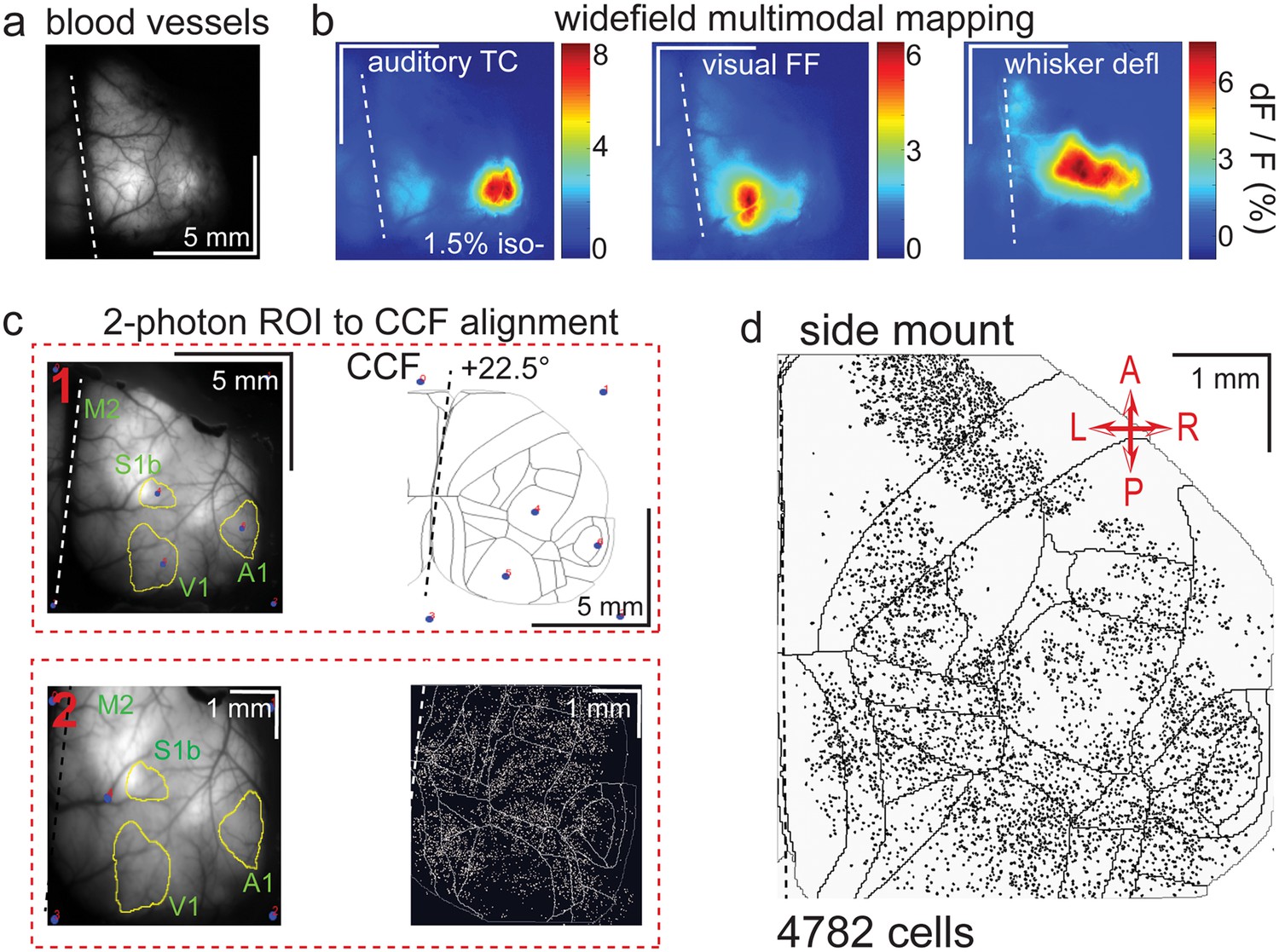
Widefield-imaging-based multimodal mapping (MMM) and CCF alignment, ROI detection, and areal assignment of GCaMP6s+ excitatory neurons for the side mount preparation.
(a) Mean projection of 30 s, 470 nm excitation fluorescence widefield movie of vasculature performed through a side mount cranial window. Midline indicated by a dashed white line. (b) Mean 1 s baseline subtracted dF/F images of 1 s responses to ~20–30 repetitions of left-side presentations of a 5–40 kHz auditory tone cloud (auditory TC; left), visual full field (FF) isoluminant Gaussian noise stimulation (center), and 100 ms x 5 Hz burst whisker deflection (right) in an example side mount preparation mouse under 1.5% isoflurane anesthesia. (c) Example two-step CCF alignment to side mount preparation, performed in Python on MMM masked blood-vessel image (upper left), rotated outline CCF (upper right), and Suite2p region of interest (ROI) output image containing exact position of all 2p imaged neurons (bottom right). Yellow outlines show the area of masks from thresholded mean dF/F image for repeated auditory, full-field visual, and/or whisker stimulation. In step 1 (top row), the CCF is transformed and aligned to the MMM image using a series of user-selected points (blue points with red numbered labels, set to matching locations on both left and right images) defining a bounding-box and known anatomical and functional locations. In step 2 (bottom row), the same process is applied to transformation and alignment of Suite2p ROIs onto the MMM with user-selected points defining a bounding box and corresponding to unique, identifiable blood-vessel positions and/or intersections. Finally, a unique CCF area name and number are assigned to each Suite2p ROI (i.e. neuron) by applying the double reverse-transformation from Suite2p cell-center location coordinates, to MMM, to CCF. (d) CCF-aligned Suite2p ROIs from an example side mount preparation with 4782 neurons identified in a single 70 min session from a mouse performing our 2-alternative forced choice (2-AFC) auditory discrimination task. TC = tone cloud, FF = full-field, defl = deflection, dF/F = change in fluorescence over baseline fluorescence, CCF = Allen common coordinate framework version 3.0, M2 = secondary motor cortex, S1b = primary somatosensory barrel cortex, A1 = primary auditory cortex, V1 = primary visual cortex, A = anterior, P = posterior, R = right, L = left.
Figure 4 with 2 supplements
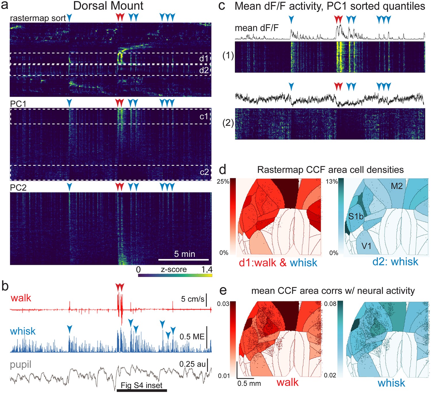
The relationship between spontaneous behavioral measures and neural activity across the dorsal cortex is globally heterogeneous.
(a) Rastermap (top), first principal component (PC1; middle), and second principal component (PC2, bottom) sorting of normalized, rasterized, neuropil subtracted dF/F neural activity for 3096 cells from a single 20-min duration example dorsal mount 2p imaging session. Each row in the display corresponds to a ‘superneuron’, or average activity of 50 adjacent neurons in the Rastermap sort (Stringer et al., 2023, bioRxiv). Activity for each superneuron is separately z-scored, then displayed as low activity in blue, intermediate activity in green, and maximum activity level in yellow (standard viridis color look-up table). Red and blue arrowheads show alignment of walking and whisking bouts, respectively, to neural activity. White dashed boxes indicate dual selections highlighted in panels (c) and (d). Scale bar shows color look-up map for each separately z-scored, individually displayed superneuron in the raster displays. (b) Behavioral arousal primitives of walk speed, whisker motion energy, and pupil diameter shown temporally aligned to the rasterized neural activity traces in (a), directly above. Horizontal black bar indicates time of expanded inset in Figure 4—figure supplement 2. (c) Expanded insets of top and bottom fifths of rasterized PC1 sorting from the middle segment of panel (a), with mean dF/F activity traces shown above each. Red and blue arrowheads indicate the same walking and whisking bouts, respectively, as in (a) and (b). (d) Normalized density of neurons in each CCF area belonging to two example Rastermap sorted groups (d1, left, red: MIN = 0%, MAX = 25%; d2, right, blue: MIN = 0%, MAX = 13%), with rasterized activities shown in corresponding labeled white dashed boxes in the top segment of panel (a). The neurons present in selected Rastermap groups are shown as Suite2p footprint outlines. The type of behavioral arousal primitive activity typically concurrently active with high neural activity for each Rastermap group is indicated below each Rastermap group’s CCF density map (i.e. walk and whisk for group d1, left (red), and whisk for group d2, right (blue)). (e) Normalized mean correlations of neural activity and walk speed (left, red; mean: MIN = 0.01, MAX = 0.03) and whisker motion energy (right, blue; mean: MIN = 0.02, MAX = 0.08) per CCF area (i.e. average correlation of all neurons in each area) are shown for this example session. Mean walk speed correlations with neural activity (dF/F) were significantly greater than zero (p<0.001, median t(3095)=3.7, single-sample t-test; python: scipy.stats.ttest_1samp) for 15 of the 19 CCF areas with at least 20 neurons present. The areas with mean correlations not significantly larger than zero were right VISam, right SSp_ll, left VIS_rl, and left AUDd. Mean whisker motion energy correlations with neural activity (dF/F) were significantly more than zero (p<0.001, median t(3095)=4.4, single-sample t-test) for 16 of the 19 CCF areas with at least 20 neurons present. The areas with mean correlations not significantly larger than zero were right VISam, left VISam, and left VISrl. PC = principal component, ME = motion energy, au = arbitrary units, M2=secondary motor cortex, S1b = primary somatosensory barrel cortex, V1 = primary visual cortex.
Figure 4—figure supplement 1
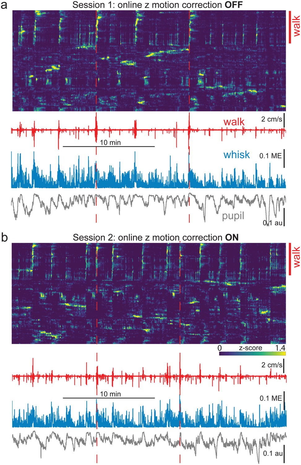
Comparison of neurobehavioral alignments with and without online z-motion correction.
Comparison of neurobehavioral alignments in back-to-back mesoscope imaging sessions either without (a, ‘OFF’) and with (b, ‘ON’) GPU-enabled online z-motion correction. (a) Neural and behavioral data are shown temporally aligned for the first session. Rastermap sorted neural activity is shown at top, with a blue/green/yellow (min/mid/max) heatmap applied to activity from each individual neuron z-scored separately. Walk speed (red), whisker motion energy (blue), and pupil diameter (gray) are shown below. Red dashed vertical lines indicate times of two major walking bouts for the purpose of alignment visualization. Note that roughly the top ~30% of neurons show strong activity time-locked to the identified walking bouts (red vertical line at right, labeled ‘walk’). (b) Same as in (a), except for a 2nd consecutive session in the same mouse. The only change was that, for this session, online GPU-enabled z-motion correction was used (“ON”) following acquisition of a 60 x 1 µm step anatomical z-stack for frame-by-frame comparison and adjustment (ScanImage/Vidrio). Note the similar percentage of cells aligned with each walking bout in the top ~30% of superneurons in Rastermap sorts in both (a) and (b) (indicated by red vertical line at right labeled ‘walk’), and the overall qualitative similarity of Rastermap clustering and activity motifs compared to that of the immediately prior session without z-motion correction shown in (a), despite the fact that these back-to-back sessions contained different detailed patterns of spontaneous activity. ME = motion energy, au = arbitrary units, GPU = graphics processing unit.
Figure 4—figure supplement 2
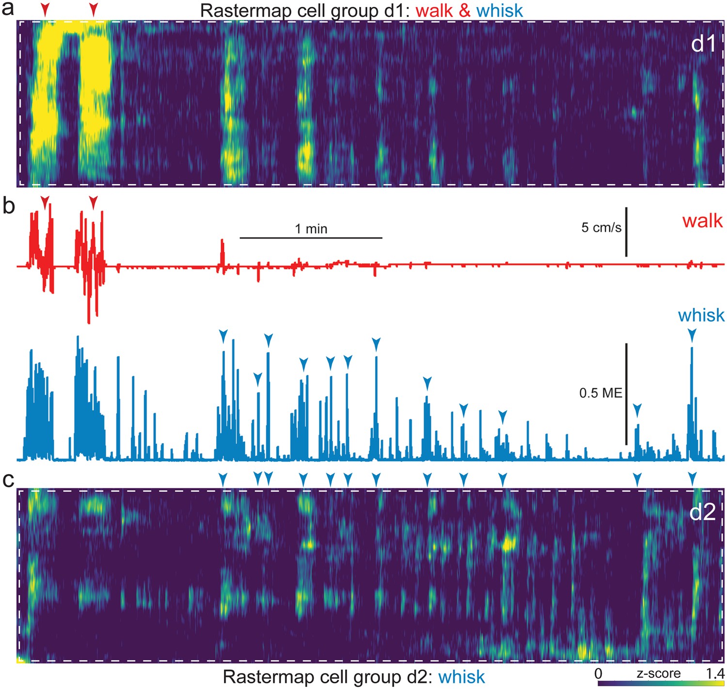
Alignment of neural activity sorted Rastermap groups and spontaneous behavior in an example dorsal mount session.
Expanded insets of Figure 4 (d1), corresponding to the walk and whisk Rastermap group (a, white dashed box) and Figure 4 (d2), corresponding to the whisk Rastermap group (c, white dashed box), shown aligned to walk speed and whisker motion energy (b, top, red, and bottom, blue, respectively). A blue/green/yellow (low/mid/high) heat map was applied to individually z-scored neural activity (a), as indicated by the scale bar (bottom right). Neural data is shown vertically temporally aligned to behavioral arousal and movement data (b). Walk speed (red) and whisker motion energy (blue) are shown for this example dorsal mount session. Red and blue arrowheads indicate temporal alignment of walk and whisk bouts, respectively, between neural and behavioral data. ME = motion energy.
Figure 5 with 2 supplements
The relationship between spontaneous behavioral measures and neural activity across the lateral cortex is regionally patterned.
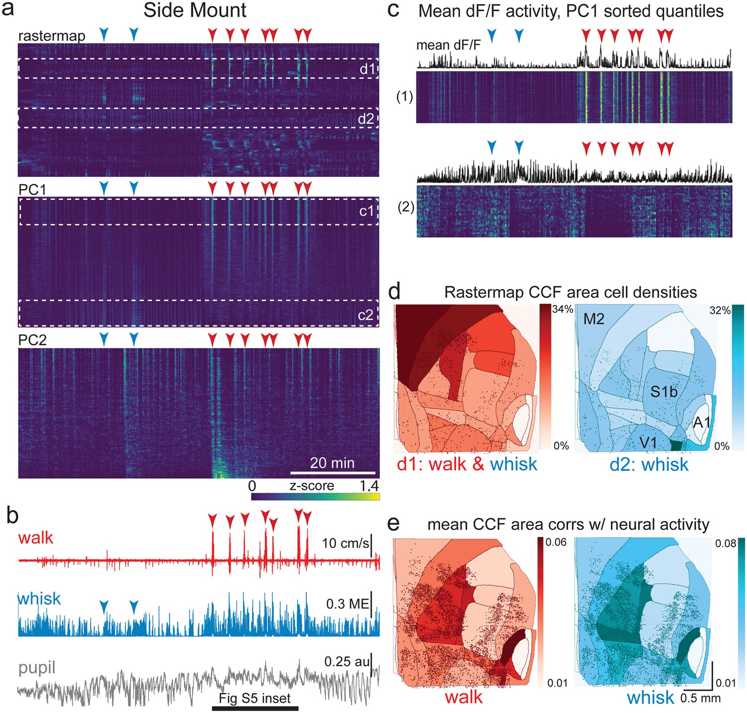
(a) Rastermap (top), first principal component (PC1; middle), and second principal component (PC2, bottom) sortings of normalized, rasterized, neuropil subtracted dF/F neural activity for 5678 cells from a single 90 min duration example side mount 2p imaging session. Each row in the display corresponds to a ‘superneuron’, or average of 50 adjacent neurons in the Rastermap sort (Stringer et al., 2023, bioRxiv). Low activity (z-scored) in blue, intermediate activity in green, maximum activity level in yellow. Red and blue arrowheads show alignment of walking and whisking bouts, respectively, to neural activity. White dashed boxes indicate selections highlighted in panels (c) and (d). Scale bar shows color look-up map for each separately z-scored, individually displayed superneuron in the raster displays. (b) Behavioral arousal primitives of walk speed, whisker motion energy, and pupil diameter shown temporally aligned to the rasterized neural activity traces in (a), directly above. (c) Expanded insets of top and bottom fifths of rasterized PC1 sorting from the middle segment of panel (a), with mean activity traces shown above each. Red and blue arrowheads indicate the same walking and whisking bouts, respectively, as in (a) and (b). Horizontal black bar indicates time of expanded inset shown in Figure 5—figure supplement 1. (d) Normalized density of neurons in each CCF area belonging to two example Rastermap sorted groups (d1, left, red: MIN = 0%, MAX = 34%; d2, right, blue: MIN = 0%, MAX = 32%), with rasterized activities shown in corresponding labeled white dashed boxes in the top segment of panel (a). Only cells in selected Rastermap groups are shown. The type of behavioral arousal primitive (i.e. walk and whisk, left, in red; whisk, right, in blue) that was typically concurrently active with high neural activity is indicated below each Rastermap group’s CCF density map. (e) Normalized mean correlations of neural activity and walk speed (left, red; mean: MIN = 0.01, MAX = 0.06; standard deviation: MIN = 0.000, MAX = 0.029) and whisker motion energy (right, blue; mean: MIN = 0.01, MAX = 0.08; standard deviation: MIN = 0.000, MAX = 0.043) per CCF area for this example session. Mean walk speed correlations with neural activity (dF/F) were significantly more than zero (p<0.001, median t(5677)=4.4, single-sample t-test; python: scipy.stats.ttest_1samp) for 20 of the 24 CCF areas with at least 20 neurons present. The areas with mean correlations not significantly larger than zero were left VISp, right SSpn, right AUDpo, and right TEa. Mean whisker motion energy correlations with neural activity (dF/F) were significantly more than zero (p<0.001, median t(5677)=7.0, single-sample t-test) for 21 of the 24 CCF areas with at least 20 neurons present. The areas with mean correlations not significantly larger than zero were right SSpn, right AUDpo, and right TEa. PC = principal component, ME = motion energy, au = arbitrary units, M2 = secondary motor cortex, S1b = primary somatosensory barrel cortex, V1 = primary visual cortex, A1 = primary auditory cortex.
Figure 5—figure supplement 1
Alignment of neural activity sorted Rastermap groups and spontaneous behavior in example side mount session.
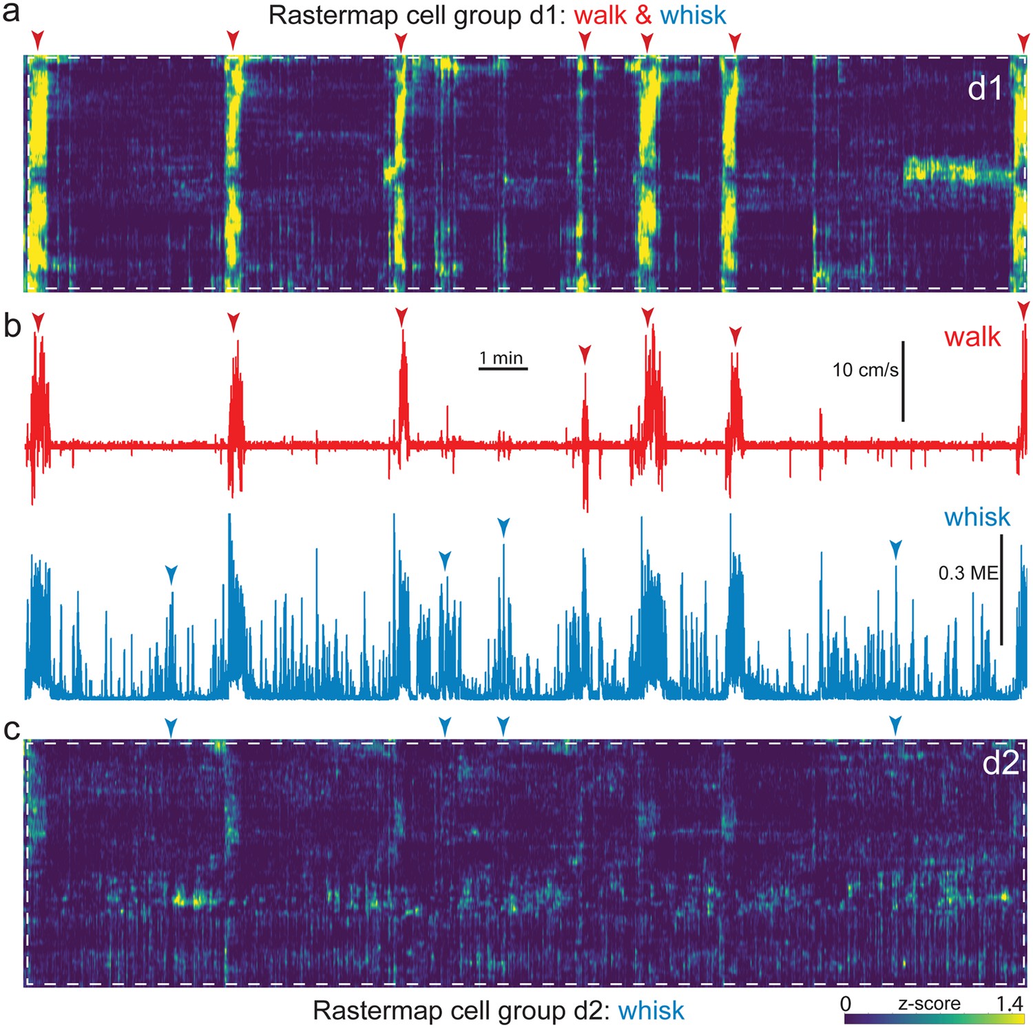
Expanded insets of Figure 5 (d1; white dashed box), corresponding to the walk and whisk Rastermap group (a), and Figure 5 (d2; white dashed box), corresponding to the whisk Rastermap group (c), shown aligned to walk speed and whisker motion energy (b, top, red, and bottom, blue, respectively). A blue/green/yellow (low/mid/high) heat map was applied to individually z-scored neural activity (a), as indicated by the scale bar (bottom right). Neural data is shown temporally aligned to behavioral arousal and movement data (b). Walk speed (red) and whisker motion energy (blue) are shown for this example side mount session. Red and blue arrowheads indicate temporal alignment of walk and whisk bouts between neural and behavioral data. ME = motion energy.
Figure 5—figure supplement 2
Heterogeneity of arousal and movement correlations with neural activity in the dorsal and side mount preparations.
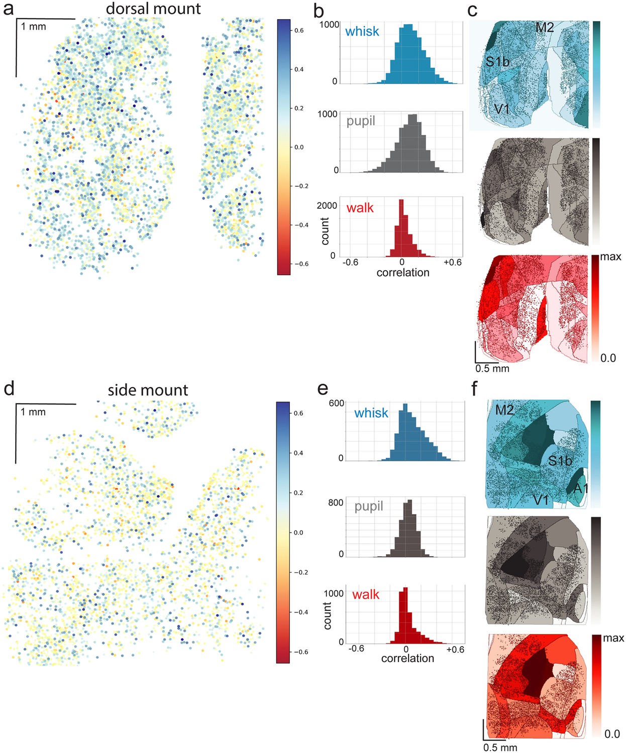
(a) Color-coded correlations of dF/F with whisker motion energy in individual neurons of the dorsal preparation in a different example session from the same mouse as in Figure 4, with large positive correlations shown in blue, large negative correlations shown in red, and small correlations shown in white/light-blue/light-red. (b) Histograms of whisk ME, pupil diameter, and walk speed (cm/s) for the same example session as in (a). (c) Normalized mean of mean correlations of neural activity with behavioral arousal primitives of whisker motion energy (blue; mean: MIN = 0.00, MAX = 0.05; standard deviation (STD): MIN = 0.002, MAX = 0.045), pupil diameter (gray; mean: MIN = 0.00, MAX = 0.06; STD: MIN = 0.004, MAX = 0.038), and walk speed (red; mean: MIN = 0.00, MAX = 0.02; STD: MIN = 0.004, MAX = 0.018) for each CCF area across eight sessions from the same dorsal mount mouse shown in Figure 4. Mean whisker motion energy correlations with neural activity (dF/F) across these eight sessions from the same mouse were significantly more than zero (p<0.05, median t(7)=3.0, single-sample t-test; python: scipy.stats.ttest_1samp) for 24 of the 27 CCF areas with at least 20 neurons present. The areas with mean correlations not significantly larger than zero were left SSp-m, SSp-n, and SSp-un. Mean pupil diameter correlations with neural activity (dF/F) were significantly more than zero (p<0.05, median t(7)=1.3, single-sample t-test) for 8 of the 27 CCF areas, including left VISp, VISam, VISpm, MOp, and SSp-ll, SSp-ul, and right VISp and SSp-ul. Mean walk speed correlations with neural activity (dF/F) were not significantly more than zero (p<0.05, median t(7)=1.0, single-sample t-test) in any of the 27 CCF areas. (d) Color-coded correlations (same lookup table as in a) of dF/F with whisker motion energy in individual neurons of the side mount preparation in an example session from the same mouse as in Figures 5 and 6. (e) Histograms of whisk ME, pupil diameter, and walk speed (cm/s) for the same example session as in (d). (f) Normalized mean of mean correlations of neural activity with behavioral arousal primitives of whisker motion energy (blue; mean: MIN = 0.00, MAX = 0.08; standard deviation (STD): MIN = 0.000, MAX = 0.043), pupil diameter (gray; mean: MIN = 0.00, MAX = 0.02; STD: MIN = 0.000, MAX = 0.034), and walk speed (red; mean: MIN = 0.00, MAX = 0.01; STD: MIN = 0.000, MAX = 0.029) for each CCF area across eight sessions from the same side mount mouse shown in Figures 5 and 6. Mean whisker motion energy correlations with neural activity (dF/F) across these eight sessions from the same mouse were significantly more than zero (p<0.05, median t(7)=5.3, single-sample t-test; python: scipy.stats.ttest_1samp) for 23 of the 23 CCF areas with at least 20 neurons present. Mean pupil diameter correlations with neural activity (dF/F) were significantly more than zero (p<0.05, median t(7)=1.2, single-sample t-test) for the right VISl and right TEa areas only. Mean walk speed correlations with neural activity (dF/F) were not significantly more than zero (p<0.05, median t(7)=1.1, single-sample t-test) in any of the 23 CCF areas.
Figure 6 with 1 supplement
Alignment of activity sorted neural ensembles and spontaneous behavioral motifs reveals sparse, distributed encoding of arousal measures across dorsolateral cortex in the side mount preparation.
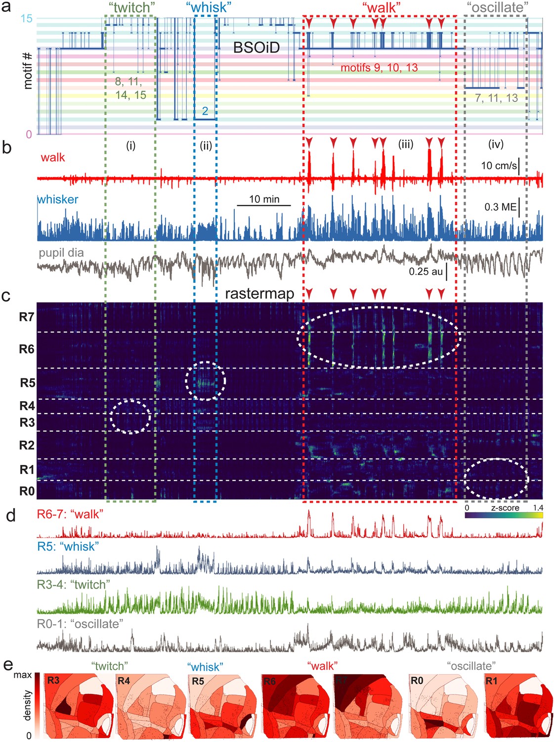
(a) Manual identification of high-level, qualitative behaviors (twitch, green dashed box; whisk, blue dashed box; walk, red dashed box; pupil oscillate, gray dashed box), aligned to sets of raw, unfiltered behavioral motifs (B-SOiD) extracted from pose-estimates (DeepLabCut) for a single example session. Numbered B-SOiD motifs (trained on a set of four sessions from the same mouse, motif # indicated by the position of the thick blue line relative to the y-axis at each time point) are color-coded (horizontal bars) across the entire 90-min session. (b) High-level behaviors (dashed colored boxes, (i–iv) and BSOiD motifs from a) are vertically temporally aligned to the behavioral primitive movement and arousal measures of walk speed, whisker motion energy, and pupil diameter. Expanded alignments of high-level behaviors ii (whisk) and iii (walk) are shown in Figure 6—figure supplement 1a, b, Red arrowheads indicate temporal alignment positions for multiple walk bouts across BSOiD motifs (a), behavioral arousal primitives (b), and Rastermap sorted neural data (c). (c) Rastermap sorted, z-scored, rasterized, neuropil subtracted dF/F neural activity (10th percentile baseline, rolling 30 s window) from the same side mount session, temporally aligned to the behavioral data directly above. Numbers at left (R0–R7) indicate Rastermap motif numbers, selected manually ‘by-eye’ for this session, and the horizontal dashed white lines on the Rastermap-sorted neural data indicate the separation between neighboring Rastermap motifs. Each row in the display corresponds to a ‘superneuron’, or average of 50 adjacent neurons in the Rastermap sort (Stringer et al., 2023, bioRxiv). Colored, dashed boxes indicate alignment of high-level behaviors with neural activity epochs from the same example session. White dashed ovals indicate areas of Rastermap group-aligned active neural ensembles during periods of defined high-level behaviors. The 2p sampling rate for this session was 3.38 Hz. (d) Normalized mean activity traces for all neurons in each neural ensemble indicated in (c) (white dashed ovals). Each trace also corresponds and is aligned to the indicated Rastermap groups. (e) Color-coded neuron densities per CCF area corresponding to Rastermap groups shown in (c), shown grouped by qualitative high-level behaviors, as indicated in (a, b). Cross-indexing with neurobehavioral alignments (white dashed ovals) in (c) allows for visualization of spatial distribution of neurons active during identified high-level behaviors (a) consisting of defined patterns of behavioral primitive movement and arousal measures (b). Corresponding maximum cell density percentages in each CCF area (white to red scale bar, top right) for each normalized Rastermap (R0–7, excluding R2) heatmap color lookup table are 11.4, 31.8, 22.9, 24.1, 38.4, 33.2, and 24.0%, respectively (left to right: R3, R4, R5, R6, R7, R0, and R1). This list of cell density percentages, therefore, corresponds to that of the CCF area filled with the darkest shade of red in each Rastermap group. White CCF areas in each Rastermap group are areas where no cells of that group were found in this example session, or where the total number of cells was less than 20 and therefore the density estimate was deemed unreliable and not reported. ME = motion energy, au = arbitrary units, CCF = common coordinate framework.
Figure 6—figure supplement 1
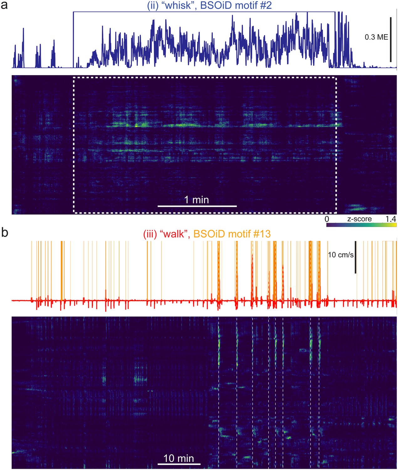
Example expanded alignment of high-level behaviors and primary corresponding BSOiD motifs, arousal measures, and Rastermap sorted neural data from side mount preparation, same example session as in Figures 5 and 6.
(a) Inset (ii) from Figure 6a, an example of active whisking (“whisk”) behavior. Whisker motion energy (solid blue line, top) is shown aligned to BSOiD motif #2 (one-hot encoded, solid blue square-wave line; up = 1 (ON), down = 0 (OFF), and Rastermap sorted neural activity (z-scored for each neuron; blue = min, green = intermediate, yellow = high) for this example session. Number of neurons = 5,678. (b) Same session and display as in a), but for inset (iii) “walk” and BSOiD motif #13 (yellow) from Figure 6a. White vertical dashed lines are aligned with major walking bouts. ME = motion energy.
Videos
Video 1
Dorsal mount.
Upper left, 3D printed titanium headpost for dorsal mount (left; i.materialise.com and sculpteo.com) and accompanying cranial window for dorsal mount (labmaker.org, or TLCInternational.com and glaswerk.com), shown in top and side orthogonal projection, followed by isometric projection (AutoDesk Inventor, Adobe Acrobat Pro 3D viewer). Upper right, 3D printed plastic (PLA) light-shields or ‘woks’, same views as upper left. Horizontal light shield (left) fits onto perimeter of dorsal mount headpost and is attached with Sylgard 170 Fast Cure silicone elastomer, and vertical light shield fits onto vertical perimeter ridge of horizontal light shield and is held by gravity. Bottom, simultaneous and temporally aligned high-resolution videography from three points-of-view of a mouse under spontaneously behaving conditions (shown at 3x speed or 90 Hz; left and right camera are GigE Teledyne Dalsa M2050 cameras, and posterior camera is FLIR grasshopper USB3 a camera). Example pose tracking labeling by DeepLabCut (Mathis et al., 2018) is shown (right camera).
Video 2
Side mount: same as in dorsal mount (Video 1), but for side mount hardware.
Note that the mouse’s headpost is retained by a single fixed support arm, rotated 22.5 degrees to the left, whereas the mouse in the dorsal mount example is held by dual orthogonally positioned fixed support arms.
Video 3
Dorsal mount multimodal mapping: example widefield (1p) imaging of GCaMP6s fluorescence responses during a visual multimodal mapping session.
Top right, full field, left-side isoluminant Gaussian noise stationary grating patches (vertical and horizontal stationary grating patches; 0.16 cpd, 30 deg; Michaiel et al., 2019) presented to elicit a visual response in right cortex, with small upper left-corner alternating white/black box positioned under photodiode to record precise stimulus presentation times. Top left, pixelwise dF/F response of the entire image for a single trial, recorded at 50 Hz and shown at 0.5 x speed. The baseline was calculated as the median of a 1 s period leading up to the stimulus onset. The dashed white circle indicates the putative primary visual cortex (right V1). A = anterior, L = left, R = right, P = posterior, dF/F = change in fluorescence divided by baseline fluorescence; midline extends vertically near the center of frame from bottom to top edge roughly between the ‘A’ and ‘P’: labels. Bottom, trace of mean dF/F for all pixels inside dashed white circle (mask), expressed as percent change. Vertical black line indicates stimulus onset. The visual stimulus is present through the end of the epoch shown. Upper left, overlay: mean of 33 dF/F responses (mean of 1 s after stimulus onset minus mean of 1 s leading up to stimulus onset) in a single dorsal mount session under 2–3% isoflurane anesthesia. ITI = inter-trial interval, measured from beginning of one stimulus to beginning of the next stimulus.
Video 4
Whisker stimulation: same as in dorsal mount multimodal mapping visual stimulation example video (Video 3), with same mouse on same day, except with 5 Hz, 100 ms duration forward swipes with custom 3D printed plastic (PLA) whisker-deflector, as indicated by vertical deflections in stimulus trace, mid-right.
Example video of mouse shown from a different session than dF/F data, because mouse face video was typically not recorded during multimodal alignment sessions. Red S1b (and dashed line) = right primary whisker barrel cortex. A = anterior, P = posterior, L = left, R = right, V1 = primary visual cortex.
Video 5
Side mount multimodal mapping: Same as in Video 3 but for side mount preparation. 1.5–3% isoflurane anesthesia was used in all 3 sessions.
Auditory: 1 s tone cloud with tones between 2 and 40 kHz presented for 0.5 s starting at black vertical dashed line (bottom). Sonogram display from Spike2 (CED) shows individual tones as horizontal green lines, where y-axis is sound frequency (~0–25 kHz) and x-axis is time (0–1 s). Movies shown at 0.25x speed. As in other example videos, the mouse shown is from a different session, but is exposed to the same stimulus at the indicated time. The mouse shown is from a different session type when videography was enabled, to show the normal response of the mouse to the stimulus. ml = midline, A1 = primary auditory cortex, A = anterior, L = left, R = right, P = posterior, dF/F = change in fluorescence divided by baseline fluorescence.
Video 6
Same as in Video 5 but for visual stimulation, with different side mount example mouse.
ml = midline, A1 = primary auditory cortex, A = anterior, L = left, R = right, P = posterior, dF/F = change in fluorescence divided by baseline fluorescence.
Video 7
Same as in Videos 5 and 6 but for whisker stimulation, with same side mount example mouse as in Video 5.
ml = midline, A1 = primary auditory cortex, A = anterior, L = left, R = right, P = posterior, dF/F = change in fluorescence divided by baseline fluorescence.
Video 8
Dorsal mount.
Titanium 3D printed headpost shown from above, with paraformaldehyde-fixed mouse brain shown beneath custom cranial window, colored Allen CCF outlines, and an example 5 x 4.62 mm mesoscope FOV corresponding to data in this video shown inside an inset box indicated by a white dashed line. Next segment, left, full 5 x 4.62 mm ScanImage (Vidrio) rendered mesoscope 2-photon field of view, rotated and flipped so that the top corresponds to the front of the mouse and the left corresponds to the left hemisphere of the cerebral cortex. Black horizontal joining lines indicate the ‘seams’ between adjacent ROIs where they are joined by rendering. The resonant scanner moves along the short axis of each rectangle, perpendicular to the ‘seams’, and mechanical galvanometers move along the long axis, parallel to the ‘seams’. Midline vertically oriented (i.e. from posterior, at bottom, to anterior, at top) blood vessel (sinus) prominent at center of frame. A movie (100 s duration shown) acquired with unidirectional scanning at 1.62 Hz, smoothed with a running average of three frames, is shown at 3x playback rate. Center top, expanded inset from white dashed box (left), shown synchronized with larger video. Bottom center, high-resolution left face videography of mouse from this session, synchronized with 2p video, rasterized neural data (upper right), and Spike2-recorded (CED) behavioral data (whisking motion energy in blue, pupil diameter in gray, and walk speed in red). Neural data was sorted in Suite2p (Stringer et al., 2019) with Rastermap (top), or by its first (middle) or second (bottom) principal component of activity over the entire session, and is displayed as z-scored (normalized) dF/F neuropil subtracted activity indexed to a single color-map lookup table with yellow as maximum, green as intermediate, and blue/purple as minimum activity level (i.e. GCaMP6s fluorescence; same lookup table scale as in Figure 4a). Red arrowheads indicate co-alignment of transient arousal increases accompanied by walking, whisking, and pupil dilation, with diverse changes in neural activity across rastermap, PC1-, and PC2-sorted ensembles.
Video 9
Example two-dimensional field of view (FOV) rendered movie and insert from an example session where factorial hidden Markov modeling showed near global synchrony of PC1 loading during walking bouts in a side mount mouse.
A 5 x 5 mm full FOV movie (~10x real-time) is shown at top left, with a 1 x 1 mm inset (white dashed box) expanded and shown at bottom left. Three example Suite2p-extracted neuron ROIs (1, 2, and 3) and a blood vessel ROI (bv) are indicated with white dashed circles. Gray traces at right indicate mean pixel fluorescence intensity of all pixels within each of these ROIs over ~450 2p movie frames. Rasterized rendering at top right indicates PC1 loading (blue/green/yellow = low/medium/high) across all CCF areas contained in the 2p movie (one per row). The red horizontal lines at the end of the shown epoch are a graphical rendering artifact that was not removed. White/gray/black rows indicate the current state of each of four hidden factors (i.e. state 0 = white, state 1 = gray, and state 2 = black) in a factorial hidden Markov model (fHMM) fit to the first 15 PCs of global neural data, the blue row indicates walk speed, the next, split blue row indicates left and right whisker pad motion energy, and the red, bottom row indicates pupil diameter. Actual behavioral arousal and movement primitives are shown as traces below (walk = red, whisk = blue, pupil = gray). Note that walk-related activity changes are correlated with independent fluctuations across the three example neurons, and furthermore that blood vessel fluctuations are small and not movement-locked, consistent with the idea that neurobehavioral activity alignment in this case, even with detected transient global synchrony across the first PC of activity, is not driven by brain movement artifact.
Video 10
Side mount.
Same as in Video 8, but for an example session from a side mount mouse instead of a dorsal mount mouse. Data from a100 s contiguous segment of single session, played at 3x original speed (3.06 Hz 2-photon acquisition, bidirectional scanning with 3-frame running average applied). Right cortex is shown (5 x 4.62 mm total at 5 µm resolution per pixel in x and y), with anterior at front (top), auditory cortex at bottom right, and midline at left edge of frame. Behavioral videography shown is taken from the right side and shows the entire front end of the mouse including torso, paws, ears and face. Time scaling is the same as in Video 8.
Video 11
Example simultaneous dual color mesoscope acquisition shows independence of activity-driven Ca2+ transients from movement artifacts.
(a), (c) Simultaneous dual color acquisition of activity-independent EYFP (top) and activity-dependent RCaMP (bottom; Thy1-RGECO). Dashed white circles indicate ROIs whose mean pixel intensities are shown in (b), (d). (b) Mean raw pixel intensity for the two ROIs shown in (a). The blue arrow indicates an example of blanking during 473 nm optogenetic stimulation (i.e. PMT is shuttered during 473 nm laser stimulation, so that section of trace is removed because it does not reflect actual fluorescence activity from the mouse cortex), and the red arrow shows an example of walking-induced movement of the imaged FOV. (d) Same as in (b), but for 3 ROIs shown in (c). Note that the magnitude of the movement artifact related transient in the Ca2+ indicator fluorescence (i.e. the red channel, PMT2) is relatively unchanged relative to adjacent peaks in ROI1, an identified neuron, and is very small or nonexistent in other neuropil and blood vessel ROIs, and in the yellow anatomical channel (PMT1). PMT = photomultiplier tube.
Tables
Appendix 1—table 1
Approximate costs–single behavior rig.
| Product description | Manufacturer | Quantity | Unit price | Extended price ($USD) |
|---|---|---|---|---|
| 25 Watt power supply | Tucker Davis | 1 | 325 | $325.00 |
| Electrostatic loudspeakers | Tucker Davis | 4 | 195 | 780.00 |
| Electrostatic loudspeaker drivers | Tucker Davis | 2 | 650 | 1,300.00 |
| PC14461 Sound card | National Instruments | 1 | 4,805.00 | 4,805.00 |
| SCB 68 with Connector Cable | National Instruments | 1 | 478.00 | 478.00 |
| PCle 6321 Multifunction I/O | National instruments | 1 | 690.00 | 690.00 |
| 810 nm narrow bandpass filter | Midwestern Optical Systems | 1 | 141 | 141 |
| Genie Nano M2050 Mono | Teledyne Dalsa | 1 | 878.43 | 878.43 |
| NE-500 Programmable OEM Syringe Pump | New Era Pumps | 7 | 495 | 3,465.00 |
| US OEM Starter kit | New Era Pumps | 7 | 25 | 175 |
| C-Mount 55 mm Telecentric Fixed Focus Lens COTEC55 | computar | 4 | 327.52 | 1,310.08 |
| Assorted Optomechanical Posts and breadboard (approximate) | Thorlabs | varied | N/A | 488.88 |
| LCD Monitor with Blanking Apparatus (Includes Arduino Micro-Controller) (approx.) | Amazon/Arduino | varied | N/A | 120.00 |
| Rotary Encoder | KAMAN AUTOMATION INC | 1 | 217 | 217.00 |
| Custom Cylindrical Treadmill | Public Missiles LTD | 1 | 84 | 84.00 |
| Lick Detection Unit | Custom Build | 1 | 1000 | 1000.00 |
| Computer for Behavior (Intel i5 or better, 32 GB RAM or better) (approx.) | User Preference | 2 | 700 | 1400.00 |
| Assorted Electrical Components, Misc. Hardware, Adapters, etc. | Varied | varied | N/A | 700.00 |
| Power 1401 | CED | 1 | 5697.60 | 5697.60 |
| Total | 24,054.99 |
Additional files
Download links
A two-part list of links to download the article, or parts of the article, in various formats.
Downloads (link to download the article as PDF)
Open citations (links to open the citations from this article in various online reference manager services)
Cite this article (links to download the citations from this article in formats compatible with various reference manager tools)
Pan-cortical 2-photon mesoscopic imaging and neurobehavioral alignment in awake, behaving mice
eLife 13:RP94167.
https://doi.org/10.7554/eLife.94167.3


