Cell-type-specific origins of locomotor rhythmicity at different speeds in larval zebrafish
- Department of Neurobiology, Northwestern University, United States
- Interdisciplinary Biological Sciences Graduate Program, Northwestern University, United States
Figures
Figure 1
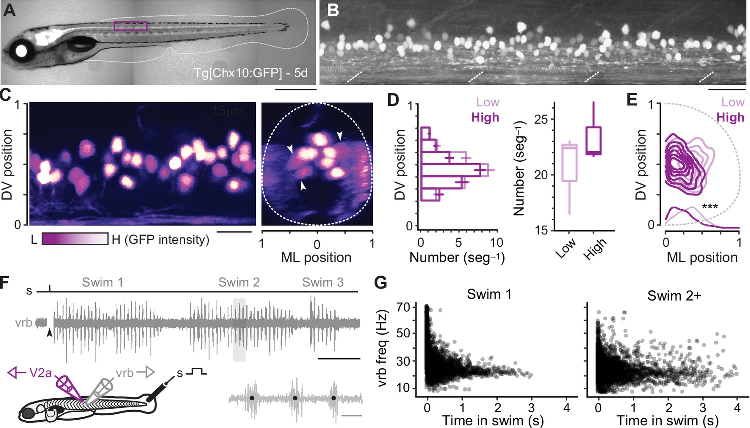
Identification of V2a neurons for recordings during ‘fictive’ swimming.
(A) Composite differential interference contrast (DIC)/epifluorescence image of Tg[Chx10:GFP] larval zebrafish at 5 days post fertilization (5d). Dorsal is up and rostral is left. Scale bar, 0.5 mm. (B) Confocal image of the Tg[Chx10:GFP] spinal cord from segments 10–15 at midbody (purple box in A). Scale bar, 30 μm. (C) Pseudo-colored images of V2a somata based on high (H, white) and low (L, purple) GFP intensity. Left panel: sagittal section, right panel: coronal section. Dashed lines indicate boundaries of spinal cord, which are normalized to 0–1 in the dorsoventral (DV) and mediolateral (ML) axes. White arrowheads indicate large, lateral V2a somata with low levels of GFP expression. Scale bar, 20 μm. (D) Plots of numbers of low- and high-intensity V2a neurons per midbody segment (n = 5–6 segments from 3 fish). Left panel: bar plot of average number (± standard error of the mean or SEM) of low and high GFP V2a neurons along the DV axis. There is no significant difference in the medians of the DV distributions of high and low GFP expressing V2a neurons (Wilcoxon rank-sum rest; W = 684, p = 0.698, n = 347 high and 401 low GFP neurons from 3 fish). Right panel: box and whisker plot showing average number of high and low GFP neurons per segment (Wilcoxon rank-sum test; W = 88, p = 0.053, n = 17 segments in 3 fish). (E) Two-dimensional contour density plots showing the ML and DV distributions of V2a neurons expressing low or high levels of GFP. Density distributions of ML positions of V2a neurons are shown at the bottom of the contour plots, which are significantly different (***, two-sample Kolmogorov–Smirnov test; D = 0.164, p < 0.001, n = 347 high and 401 low GFP neurons from 3 fish). (F) Top panel: an example of an extracellular ventral rootlet recording of three consecutive swim episodes evoked by a mild electrical stimulus (s) to the tail fin (at arrowhead, artifact blanked). Scale bar, 500 ms. Bottom left panel: a cartoon of the locations of the stimulus and the recording electrodes. Bottom right panel: individual ventral rootlet bursts (vrb) on an expanded timescale. Black dots mark the center of each vrb used to calculate swim frequency in Hz (1/s), which is indicative of swimming speed. Scale bar, 20 ms. (G) Scatter plot of vrb frequency (Hz) versus the time in swim episode (ms). The swimming episode immediately following the stimulus is called Swim 1 (left), and any subsequent swimming episodes are called Swim 2+ (right).
Figure 2
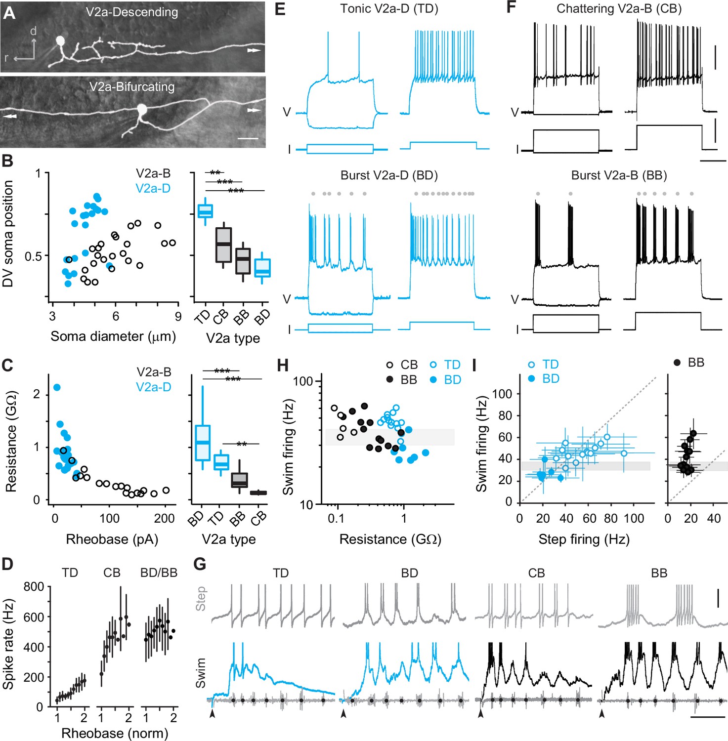
Cell-type-specific electrophysiological properties linked to recruitment order.
(A) Composite DIC/epifluorescent images of post hoc fills of V2a-Descending (V2a-D, top) and V2a-Bifurcating (V2a-B, bottom) neurons. Arrows indicate continuation of axons outside the field of view. Scale bar, 10 μm. (B) Left panel: scatter plot of soma diameter of V2a-D and V2a-B neurons normalized to dorsoventral (DV) soma position, with 1 demarcating the dorsal and 0 the ventral boundaries of the spinal cord. The soma diameters of V2a-Ds (n = 22) and V2a-Bs (n = 25) are significantly different according to the Wilcoxon rank-sum test (W = 401, p < 0.001). Right panel: box plots of DV soma positions of V2a-D and V2a-B neurons classified as tonic, bursting, or chattering based on their step-firing responses in panels E and F. TD = tonic V2a-D (n = 14), CB = chattering V2a-B (n = 12), BB = bursting V2a-B (n = 13), BD = bursting V2a-D (n = 8). The differences in the DV soma positions of TD and CB (z = −3.202, p < 0.01), TD and BB (z = −4.714, p < 0.001), and TD and BD (z = −4.892, p < 0.001) are significantly different according to Dunn’s test following post hoc Benjamini–Hochberg correction. (C) Left panel: scatter plot of input resistance (GΩ) versus the rheobase (pA) of V2a-B (black) and V2a-D (blue) neurons. The input resistance (W = 30, p < 0.001) and rheobase (W = 361.5, p < 0.001) of V2a-Bs (n = 18) and V2a-Ds (n = 21) are significantly different according to the Wilcoxon rank-sum test. Right panel: box plots of input resistance (GΩ) of BD (n = 7), TD (n = 14), BB (n = 11), and CB (n = 7) V2a neurons. The differences in the input resistance of BD and BB (z = −3.531, p < 0.001), BD and CB (z = 4.734, p < 0.001), and CB and TD neurons (z = −3.559, p < 0.01) are significantly different according to Dunn’s test following post hoc Benjamini–Hochberg correction. (D) Mean (± standard deviation [SD]) instantaneous spike rates (Hz) between 1 and 2x rheobase for TD, CB, BD, and BB neurons. (E) Top panel: step-firing responses of V2a-D neurons defined as tonic (TD). Bottom panel: step-firing responses of V2a-D neurons defined as bursting (BD). Gray dots depict the midpoint of slower membrane oscillations driving the bursting spiking behavior. Same scale as panel F. (F) Top panel: step-firing responses of V2a-B neurons defined as chattering (CB). Bottom panel: V2a-B neurons defined as bursting (BB). Gray dots depict the midpoint of slower membrane oscillations driving the bursting spiking behavior. Scale bars, 20 mV, 200 pA, 200 ms. (G) Top panels: step-firing responses close to rheobase of TD, BD, CB, and BB neurons. Bottom panels: swim-firing responses evoked by a mild electrical shock shown on the same time scales. Black dots on ventral root bursts (gray) indicate swim frequency. Black arrows mark the stimulation artifact. Scale bars, 10 mV, 50 ms. (H) Scatter plot of median swim-firing frequency (Hz) versus the input resistance (GΩ) of CB, TD, BB, and BD on logarithmic x- and y-scales. Shaded gray box indicates 30–40 Hz range reflecting transition between anguilliform and carangiform swim modes. There is a significant negative correlation between the median swim-firing frequency and input resistance of TD and BD V2a neurons (Spearman’s rank correlation test, rs = −0.723, p < 0.001, n = 21) as well as CB and BB V2a neurons (rs = −0.624, p < 0.01, n = 18). (I) A comparison of median swim-firing and median step-firing frequencies between 1 and 2x rheobase (± SD) for TD, BD, and BB neurons. For TD neurons, step frequencies represent spike rates, while for BD and BB neurons they represent burst rates. CB neurons were too variable in step-firing frequency to obtain reliable median values. Shaded gray box indicates 30–40 Hz range reflecting transition between anguilliform and carangiform swim modes. There is a significant positive correlation between the median swim-firing and median step-firing frequencies of TD and BD neurons (Spearman’s rank correlation test; rs = 0.768, p < 0.001, n = 21), but not BB neurons (Spearman’s rank correlation test; rs = 0.318, p = 0.289, n = 13). Statistically significant differences are denoted as follows: *p < 0.05; **p < 0.01; ***p < 0.001.
Figure 3
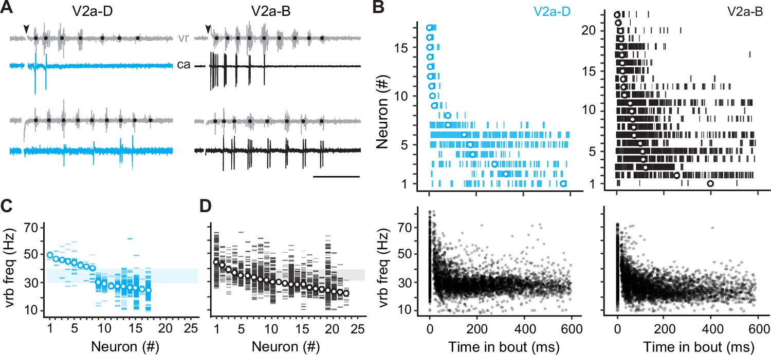
Differences in recruitment patterns among the distinct V2a types.
(A) Left panel: cell-attached (ca) recordings of descending V2a (V2a-D) neurons during fictive swimming evoked by a brief stimulus (at black arrowhead). Black dots on ventral root (vr) bursts (gray) indicate swim frequency. The top neuron fires immediately after the stimulus during high-frequency swimming, while the bottom neuron fires near the end of the episode at lower frequencies. Right panel: as shown to the left, but for bifurcating V2a (V2a-B) neurons. Scale bar, 100 ms. (B) Top panel: spike timing of V2a-D (left) and V2a-B (right) neurons relative to the start of swimming ordered by the median of the distribution. Bottom panel: a scatterplot of vrb frequency (Hz) as a function of time for all episodes (Swim 1 and 2+) during which the V2a-D (left) or V2a-B (right) neurons were recruited. (C) Raster plots of ventral root burst frequencies (Hz) over which V2a-Ds were recruited ordered by the median vrb recruitment frequency (Hz). Shaded box indicates 30–40 Hz range reflecting transition between anguilliform and carangiform swim modes. (D) Raster plots of ventral root burst frequencies (Hz) over which V2a-Bs were recruited ordered by the median vrb recruitment frequency (Hz). Shaded box indicates 30–40 Hz range reflecting transition between anguilliform and carangiform swim modes.
Figure 4
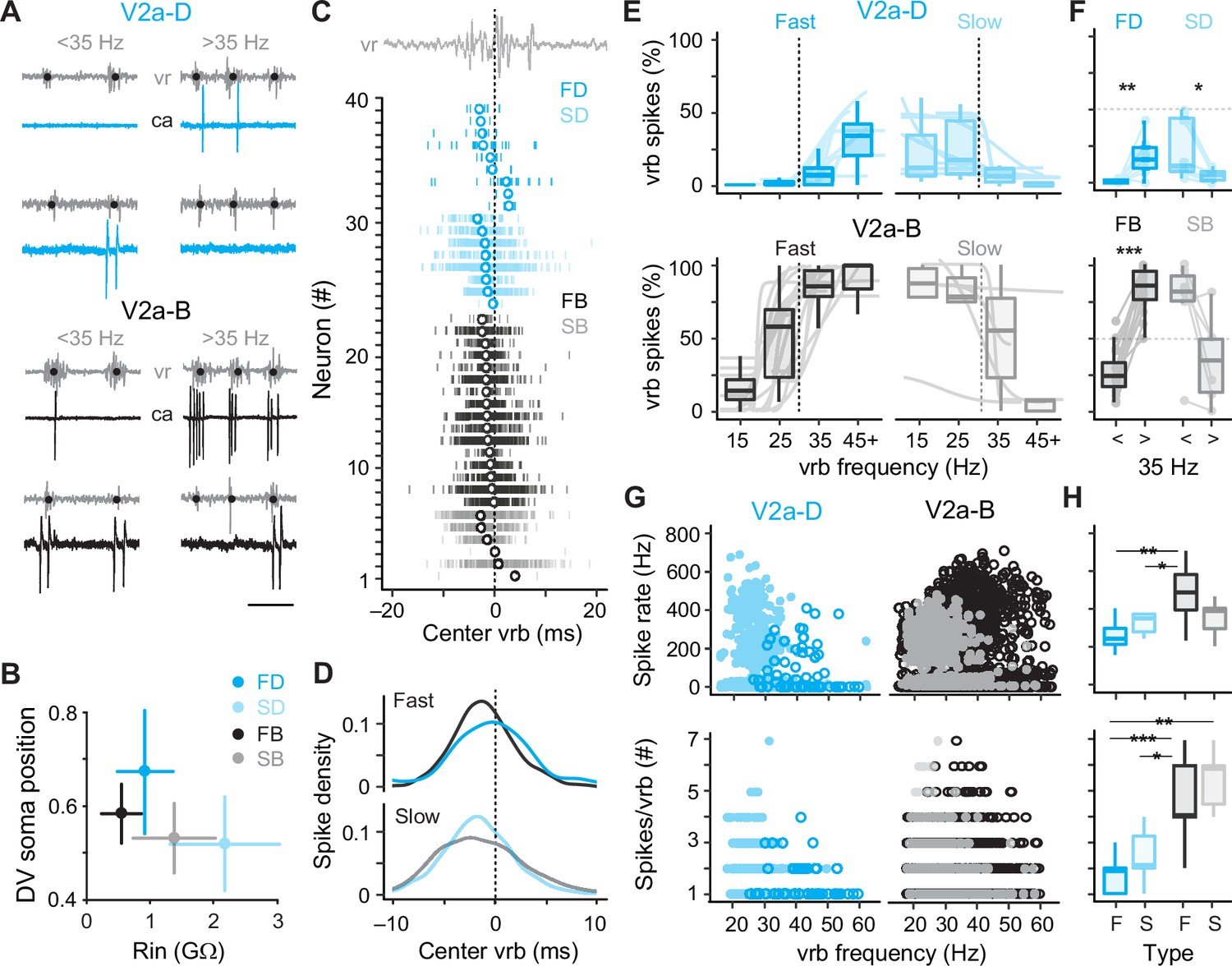
Distinct types of slow and fast V2a neurons distinguished based on recruitment.
(A) Top panel: cell-attached (ca) and ventral rootlet (vr) recordings during slow (<35 Hz) and fast (>35 Hz) swimming illustrate V2a-D neurons (blue) that fire exclusively at slow and fast speeds. Bottom panel: V2a-B neurons (black) fire more reliably at both slow and fast speeds. Scale bar, 25 ms. (B) Plots of the mean (± standard deviation [SD]) dorsoventral (DV) positions of fast (FD) and slow (SD) V2a-Ds, and fast (FB) and slow (SB) V2a-Bs versus their mean (± SD) input resistance (Rin). (C) Spike timing of slow (S) and fast (F) V2a-D and V2a-B neurons relative to the center of the ventral root burst (vrb) depicted by the dashed vertical line. Tick marks represent individual spikes from multiple cycles and circles represent median spike timing. (D) Density plots of spike timing relative to the center burst for slow and fast V2a-B and V2a-D neurons illustrated in panel C. (E) Top panel: box plots of the percentage of ventral root bursts with spikes (vrb spikes %) as a function of vrb frequency (Hz) for fast (FD, n = 9) and slow (SD, n = 8) V2a-D neurons. For box plots, the ventral root burst frequency was binned at 15 Hz intervals starting at 15 Hz, and the final interval of 45+ Hz consisted of a 20-Hz range spanning from 45 to 65 Hz. Box plots are superimposed on trendlines from individual neurons fit to data binned at 5 Hz intervals, whose slopes define whether they are fast (positive) or slow (negative). Dashed line indicates transition between slow carangiform and fast anguilliform modes. Bottom panel: as above but for fast (FB, n = 16) and slow (SB, n = 6) V2a-B neurons. (F) Top panel: box plots of vrb spikes % for slow and fast V2a-D neurons from panel E collapsed into single slow (<35 Hz) and (>35 Hz) bins for purposes of statistical analysis (Wilcoxon signed-rank test; FD, V = 1, p < 0.01, n = 9; SD, V = 36, p = <0.01, n = 8). Bottom panel: as above but for V2a-B neurons (Wilcoxon signed-rank test; FB, V = 0, p < 0.001, n = 16; SB, V = 20, p = 0.063, n = 6). (G) Top panel: scatter plots of instantaneous spike rates versus vrb frequency (Hz) for V2a-D (left) and V2a-B (right) neurons color coded as fast (dark) and slow (light). FD, n = 9; SD, n = 8; FB, n = 16; SB, n = 6. Bottom panel: scatter plots of the number of spikes per ventral root burst (#) as a function of vrb frequency (Hz), organized and color coded as above. (H) Top panel: box plots of maximum instantaneous spike rates for fast (n = 5) and slow (n = 7) V2a-D and fast (n = 16) and slow (n = 5) V2a-B neurons. Note, only a subset of V2a neurons that fired two or more spikes per cycle were included in this analysis (Wilcoxon rank-sum test; FB-FD, W = 73, p < 0.01; FB-SD, W = 90, p < 0.05). Bottom panel: box plots of the maximum number of spikes/vrb (Wilcoxon rank-sum test; FB-FD, W = 133, p < 0.001; FB-SD, W = 100, p < 0.05; FD-SB, W = 50, p < 0.01; FD, n = 9; SD, n = 8; FB, n = 16; SB, n = 6). Statistically significant differences are denoted as follows: *p < 0.05; **p < 0.01; ***p < 0.001.
Figure 5
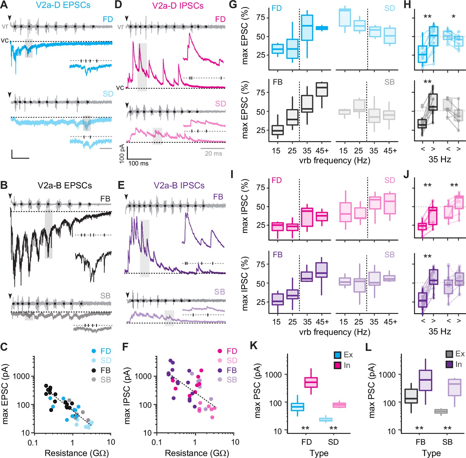
Differences in levels of synaptic drive related to speed and V2a cell type.
(A) Voltage-clamp (vc) recordings of excitatory post-synaptic currents (EPSCs) received by fast (top, FD) and slow (bottom, SD) V2a-D neurons along with ventral root (vr) recordings during fictive swimming triggered by an electrical stimulus (black arrowheads, artifact blanked). Black dots indicate burst intervals for frequency measures. Gray shaded boxes indicate region expanded inset, illustrating the holding potential (dashed line, −75 mV) and individual EPSCs (tick marks). Scale bars, 25 pA, 100 ms (20 ms inset). (B) As in A, but for fast (top, FB) and slow (bottom, SB) V2a-B neurons. (C) Scatter plot of maximum EPSC amplitude (pA) as a function of input resistance (GΩ) on logarithmic x- and y-scales. Dashed logarithmic trendlines are included for illustrative purposes (Spearman’s rank correlation test, rs = −0.873, p < 0.001, n = 39). (D) Voltage-clamp recordings of inhibitory post-synaptic currents (IPSCs) at a holding potential of 10 mV from fast (top, FD) and slow (bottom, SD) V2a-D neurons, organized as detailed in panel A. Scale bars, 100 pA, 100 ms (20 ms inset). (E) As in D, but fast (top, FB) and slow (bottom, SB) V2a-B neurons. (F) Scatter plot of maximum IPSC amplitude as a function of input resistance (GΩ) on logarithmic x- and y-scales (Spearman’s rank correlation test; rs = −0.633, p < 0.001, n = 36). (G) Top panel: box plots of the maximum EPSC per cycle as a percentage of the maximum current (max EPSC%) for fast (FD, n = 9) and slow (SD, n = 6) V2a-D neurons, organized into four bins based on frequency. Dashed line indicates transition between slow carangiform and fast anguilliform modes. Bottom panel: as above, but for fast (FB, n = 11) and slow (SB, n = 5) V2a-B neurons. (H) Top panel: Box plots of max EPSC% for fast and slow V2a-D neurons from panel G, collapsed into single slow (<35 Hz) and fast (>35 Hz) bins for purposes of statistical analysis (Wilcoxon signed-rank test; FD, V = 0, p < 0.01, n = 9; SD, V = 21, p < 0.05, n = 6). Bottom panel: As above but for V2a-B neurons (Wilcoxon signed-rank test; FB, V = 2, p < 0.01, n = 11; SB, V = 15, p = 0.063, n = 5). Boxed plots are superimposed on trendlines from individual neurons. Note, one cell each for V2a-D and V2a-B slow subtypes behaved more like fast subtypes (dashed lines). (I) Top panel: box plots of the maximum IPSC per cycle as a percentage of the maximum current (max IPSC%) for fast (FD, n = 7) and slow (SD, n = 7) V2a-Ds organized as in panel G. Bottom panel: as above but for fast (FB, n = 12) and slow (SB, n = 6) V2a-B neurons. (J) Top panel: box plots of max IPSC% for fast and slow V2a-D neurons from panel I, collapsed into single slow (<35 Hz) and fast (>35 Hz) bins for purposes of for statistical analysis (Wilcoxon signed-rank test; FD, V = 0, p < 0.05, n = 7; SD, V = 1, p < 0.05, n = 7). Bottom panel: as above, but for fast and slow V2a-B neurons (Wilcoxon signed-rank test; FB, V = 0, p < 0.001, n = 12; SB, V = 4, p = 0.219, n = 6). (K) Box plots of maximum excitatory and inhibitory current for FD (Wilcoxon signed-rank test; V = 0, p < 0.01, n = 9 for excitation, n = 8 for inhibition) and SD (Wilcoxon signed-rank test; V = 0, p < 0.05, n = 8 for excitation, n = 7 for inhibition) neurons. (L) As in K but for FB (Wilcoxon signed-rank test; V = 1, p < 0.001, n = 16 for excitation, n = 15 for inhibition) and SB (Wilcoxon signed-rank test; V = 0, p < 0.05, n = 6 for excitation, n = 6 for inhibition) neurons. Statistically significant differences are denoted as follows: *p < 0.05; **p < 0.01; ***p < 0.001.
Figure 6
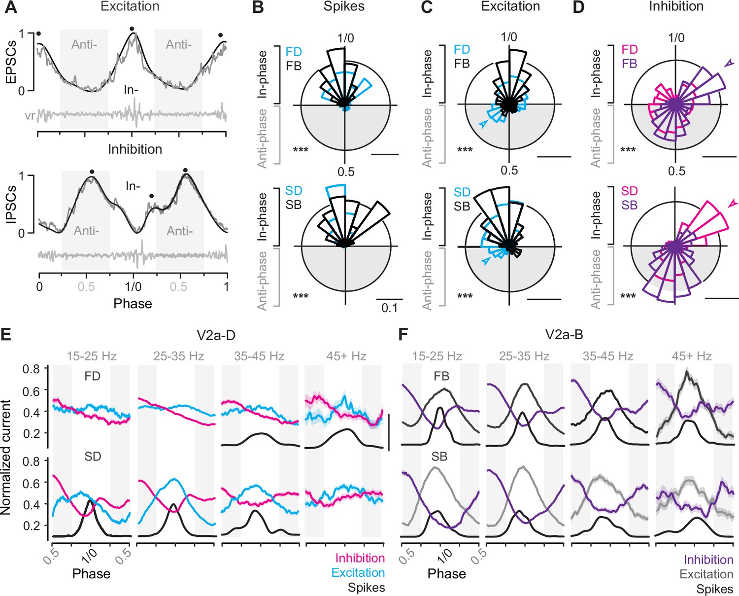
Differences in timing of synaptic drive related to speed and V2a cell type.
(A) Raw (gray) and low-pass filtered (black) traces of post-synaptic current (PSC), normalized to the peak (1) and trough (0) of phasic excitation (left) and inhibition (right). Corresponding ventral root (vr) bursts used to define in- and anti-phase (gray shaded boxes) currents are shown below. Block dots denote the peaks identified by the findpeaks() function in MATLAB. Note, excitation has been inverted to simplify comparisons to inhibition. (B) Top panel: circular bar plots of spike phase for fast descending (FD, n = 9) and bifurcating (FB, n = 16) V2a neurons (Watson’s two-sample test of homogeneity; F = 0.483, p < 0.001). Bottom panel: circular bar plots of spike phase for slow descending (SD, n = 8) and bifurcating (SB, n = 6) neurons (Watson’s two-sample test of homogeneity; F = 3.711, p < 0.001). Scale bars, 10% total distribution. (C) Top panel: circular bar plots of phase normalized peaks in low pass filtered excitatory post-synaptic currents (EPSCs) for fast descending (FD, n = 9) and fast bifurcating (FB, n = 11) V2a neurons (Watson’s two-sample test of homogeneity; F = 5.941, p < 0.001). Bottom panel: circular bar plots of phase normalized peaks in low pass filtered EPSCs for slow descending (SD, n = 7) and slow bifurcating (SB, n = 6) neurons (Watson’s two-sample test of homogeneity; F = 2.548, p < 0.001). Scale bars, 10% total distribution. (D) Top panel: circular bar plots of phase normalized peaks in low pass filtered inhibitory post-synaptic currents (IPSCs) for fast descending (FD, n = 7) and fast bifurcating (FB, n = 12) neurons (Watson’s two-sample test of homogeneity; F = 3.646, p < 0.001). Arrowhead indicates prominent in-phase IPSC component for fast V2a-Bs. Bottom panel: circular bar plots of phase normalized peaks in low pass filtered IPSCs for slow descending (SD, n = 7) and slow bifurcating (SB, n = 6) neurons (Watson’s two-sample test of homogeneity; F = 5.426, p < 0.001). Scale bars, 10% total distribution. Arrowhead indicates prominent in-phase IPSC component for slow V2a-Ds. Scale bars, 10% total distribution. (E) Line plots from V2a-D neurons of averaged excitation (Ex; FD, n = 9; SD, n = 6), averaged inhibition (In; FD, n = 7; SD, n = 7), and spike densities (S; FD, n = 7; SD, n = 7) broken into four ventral root burst frequency (Hz) bins. Post-synaptic current was normalized on a cycle-by-cycle basis, such that the minimum and maximum current per cycle equaled 0 and 1, respectively. Scale bar for spike densities, 50% total distribution. (F) As in panel E, but averaged excitation (Ex; FB, n = 11; SB, n = 5), inhibition (In; FB, n = 12; SB, n = 6), and spike densities (S; FB, n = 16; SB, n = 6) for V2a-B neurons.
Figure 7
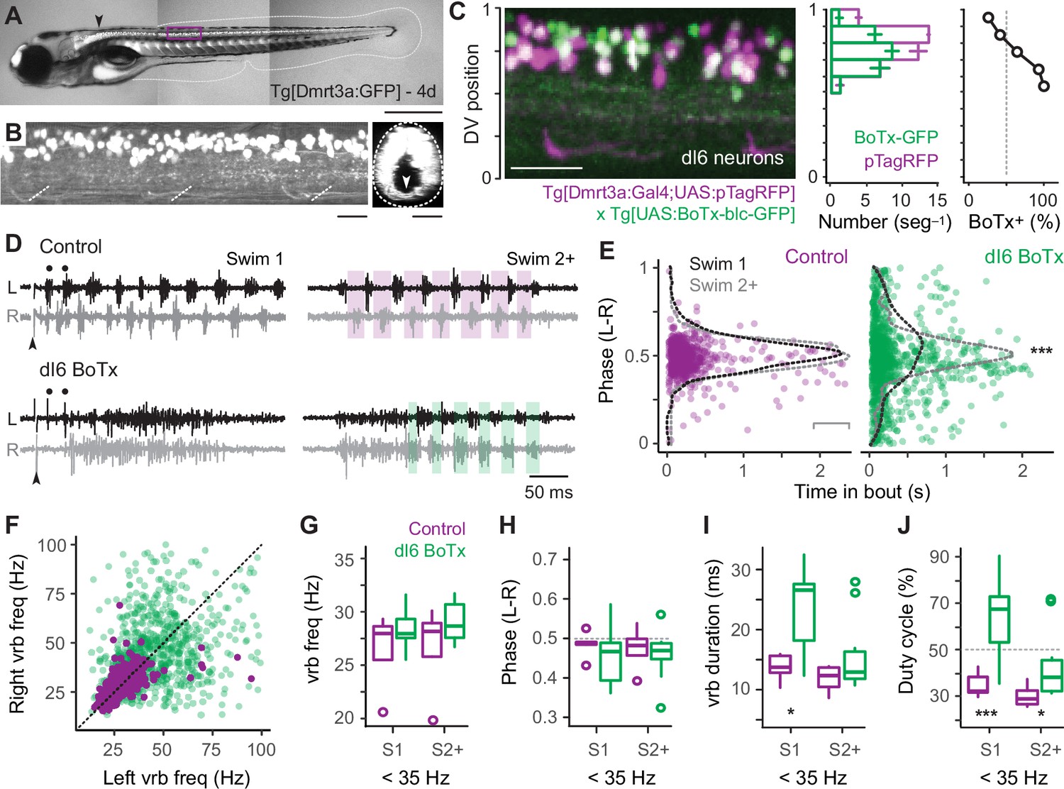
Speed-dependent impact of silencing dI6 neurons on rhythm versus pattern.
(A) Composite DIC/epifluorescence image of Tg[Dmrt3a:GFP] larval zebrafish at 4 days post fertilization (4d). Dorsal is up and rostral is left. Scale bar, 0.5 mm. (B) Left panel: confocal image of the Tg[Dmrt3a:GFP] spinal cord from segments 10–12 at midbody (purple box in A). Scale bar, 20 μm. Right panel: coronal view of confocal image to the left illustrating commissural axons of dI6 neurons (white arrowhead). Dashed lines indicate boundaries of spinal cord. Scale bar, 20 μm. (C) Left panel: composite confocal image of all dI6 somata labeled with pTagRFP (purple) and subsets of dI6 somata labeled with botulinum toxin-tagged GFP (green), using a combination of compound transgenic lines (noted below). Boundaries of spinal cord are normalized to 0–1 in the dorsoventral (DV) axis. Scale bar, 30 μm. Middle panel: bar plots of average numbers (± SEM) of pTagRFP-labeled dI6 neurons (purple) and BoTx-GFP-labeled dI6 neurons (green) per midbody segment (n = 5–6 segments from 3 fish) along the DV axis. The DV distributions of pTagRFP expressing (n = 517) and BoTx-GFP expressing dI6 neurons (n = 842) are significantly different (Wilcoxon rank-sum test; W = 184,452, p < 0.001). Right panel: line plot of percentage of total dI6 neurons labeled with BoTx-GFP along the DV axis. Dashed gray line indicates 50% of the distribution. (D) Top panels: examples of extracellular ventral rootlet recordings recorded on the left (L) and right (R) sides in sibling control larvae lacking BoTx-GFP expression. Two consecutive swim episodes are illustrated, the first (Swim 1) is evoked by a mild electrical stimulus (s) to the tail fin (at arrowhead, artifact blanked), with subsequent episodes occurring intermittently after the first (Swim 2+). Scale bar, 500 ms. Bottom panels: examples from BoTx-GFP fish with coincident bilateral activity. Black dots illustrate ipsilateral bursts that match frequencies observed in controls. Shaded purple and green boxes illustrate left–right alternation. (E) Left panel: scatter plot of left–right (L–R) phase versus the time in the swim episode (s) in control siblings. Superimposed on pooled data are density plots from the swimming episode immediately following the stimulus (Swim 1) and subsequent swim episodes (Swim 2+), which are not significantly different following a two-sample Kolmogorov–Smirnov test (D = 0.084, p = 0.305, n = 330 cycles for Swim 1 from 5 fish and 219 cycles for Swim 2+ from 4 fish). Right panel: scatter plot of BoTxBLC-GFP fish illustrating collapse of left–right alternation and rhythmicity primarily at the beginning of the swimming episodes. In this case, density plots for Swim 1 versus Swim 2+ are significantly different (***, two-sample Kolmogorov–Smirnov test; D = 0.163, p < 0.001, n = 428 cycles for Swim 1 from 11 fish and 540 cycles for Swim 2+ from 10 fish). (F) Scatter plot analyzing ventral root burstlet (vrb) frequency for control (purple) and BoTx-GFP fish (green) on the left and right sides on a cycle-by-cycle basis. (G) Box plots of ventral rootlet burstlet frequency for control and BoTx-GFP fish during carangiform swimming below 35 Hz for Swim 1 (Wilcoxon rank-sum test; W = 35, p = 0.454, n = 11 BoTx-GFP and 5 control fish) and Swim 2+ (W = 26, p = 0.453, n = 10 BoTx-GFP and 4 control fish). (H) Box plots of ventral rootlet burstlet left–right phase for control and BoTx-GFP fish during carangiform swimming below 35 Hz for Swim 1 (Wilcoxon rank-sum test; W = 18, p = 0.439, n = 11 BoTx-GFP and 5 control fish) and Swim 2+ (W = 17, p = 0.733, n = 10 BoTx-GFP and 4 control fish). (I) Box plots of ventral rootlet burstlet duration for control and BoTx-GFP fish during carangiform swimming below 35 Hz for Swim 1 (Wilcoxon rank-sum test; *, W = 48, p < 0.05, n = 11 BoTx-GFP and 5 control fish) and Swim 2+ (W = 27, p = 0.374, n = 10 BoTx-GFP and 4 control fish). (J) Box plots of ventral rootlet burstlet duty cycle for control and BoTx-GFP fish during carangiform swimming below 35 Hz for Swim 1 (Wilcoxon rank-sum test; **, W = 52, p < 0.01, n = 11 BoTx-GFP and 5 control fish) and Swim 2+ (*, W = 27, p < 0.05, n = 10 BoTx-GFP and 4 control fish). Statistically significant differences are denoted as follows: *p < 0.05; **p < 0.01; ***p < 0.001.
Figure 8
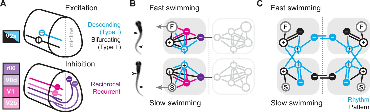
Summary diagrams of cell-type-specific origins of locomotor rhythmicity.
(A) Schematic illustrating the major spinal interneuron types that provide excitation (top) and inhibition (bottom) during locomotion. Dorsal is up and rostral is left. See Discussion for details. (B) Schematic illustrating the potential wiring diagrams between major spinal interneuron types (+, excitatory; −, inhibitory) for fast swimming (top) and slow swimming (bottom). Snapshots from high-speed videos are illustrated to the left for fast anguilliform and slow carangiform swimming. F, fast motor pools; S, slow motor pools. Dashed vertical line is midline. Reciprocal populations are shaded gray for simplicity. (C) Schematic focusing on the major connections that differentiate fast and slow swimming circuits. Rhythm-generating circuitry is in blue and pattern-forming circuitry is in black.
Videos
Video 1
High-speed video of real escape swimming in a 5-day-old larva.
(A) Larva is touched near the head by a sharpened tungsten pin, which triggers a rapid escape bend, followed by high-frequency anguilliform swimming and then ending with low-frequency carangiform swimming. Video was captured at 2000 frames per second and has been slowed down 40× for purposes of visualization (playback at 50 frames per second).
Additional files
Download links
A two-part list of links to download the article, or parts of the article, in various formats.
Downloads (link to download the article as PDF)
Open citations (links to open the citations from this article in various online reference manager services)
Cite this article (links to download the citations from this article in formats compatible with various reference manager tools)
Cell-type-specific origins of locomotor rhythmicity at different speeds in larval zebrafish
eLife 13:RP94349.
https://doi.org/10.7554/eLife.94349.3


