Spectral decomposition unlocks ascidian morphogenesis
- Northwestern University, United States
- NSF-Simons Center for Quantitative Biology, United States
- University of Montpellier, France
- LIRMM, France
- CNRS, France
- University of Chicago, United States
Figures
Figure 1
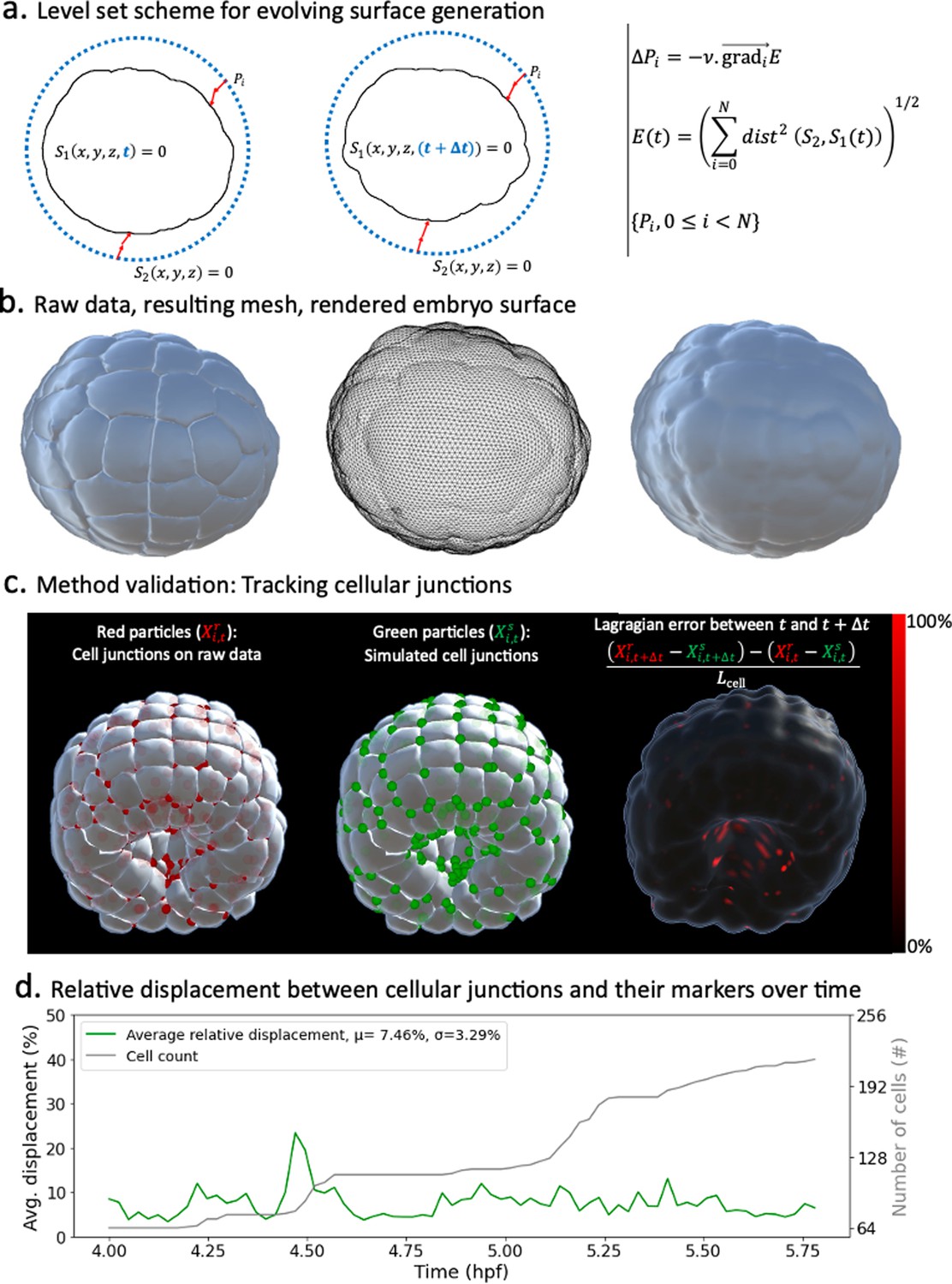
Level sets-inspired Lagrangian markers.
(a) Left: schematics of the level set method. Right: fundamentals of the numerical scheme that shapes into . (b) Illustration of the method in action. Left: raw data consisting of geometric meshes of single cells spatially organized into the embryo. Center: embryo surface mesh resulting from the application of the level set scheme. Right: rendering of the embryonic surface. (c) Tracking of cellular junctions. Left: identification of cellular junctions (red dots). Center: corresponding markers (green dots), defined as vertices on the computed embryonic surface closest to the junctions. Right: relative displacement between junctions and their markers at consecutive timepoints. (d) Plot over time of the relative displacement between cellular junctions and their markers.
Figure 2
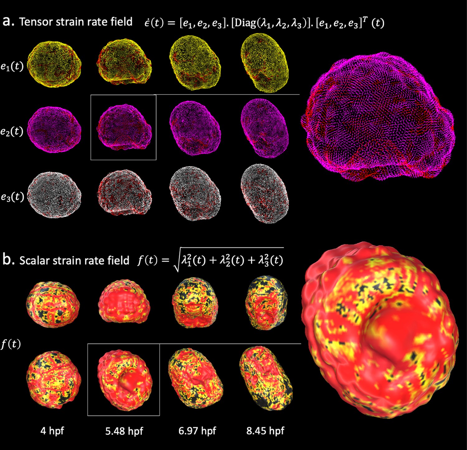
Strain rate field describes morphogenesis.
The strain rate tensor field measures the rate at which morphological changes occur in the embryo as a function of time. The strain rate tensor field is locally represented as a 3 × 3 symmetric matrix and is completely determined by its eigenvector fields. (a) Heatmap of the eigenvector fields of the strain rate tensor. Each row represents a vector field distinguished by a distinct root color (yellow, pink, white). The gradient from the root color to red represents increasing magnitudes of the strain rate tensor. Top: spatiotemporal dynamics of the first eigenvector field. Middle: spatiotemporal dynamics of the second eigenvector field. Bottom: spatiotemporal dynamics of the third eigenvector field. (b) Heatmap of the scalar strain rate field. The gradient from yellow to red depicts regions of increasing morphological activity, while black stands for areas of low morphological activity. The heatmaps show high morphological activity in the invaginating endoderm and zippering neural plate, but also across the embryonic animal during rounds of synchronised division.
Figure 3
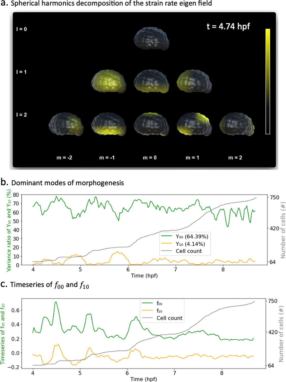
Spherical harmonics decomposition of morphogenesis.
(a) Example of spherical harmonics decomposition of the scalar strain rate field mapped to the embryo at hpf. Each picture represents the value of the harmonic field () multiplied by its coefficient . here are taken relative to each specific minimal and maximum bounds in the entire time window of observation. Thresholding is applied for better rendering. (b) Time evolution of the variance ratios of the main modes of ascidian early morphogenesis ( and ). The cell population dynamic is also included in the plot for clarity. (c) Time evolution of the coefficients and associated with spherical harmonics ( and ). The cell population count is also included in the plot for clarity.
Figure 4
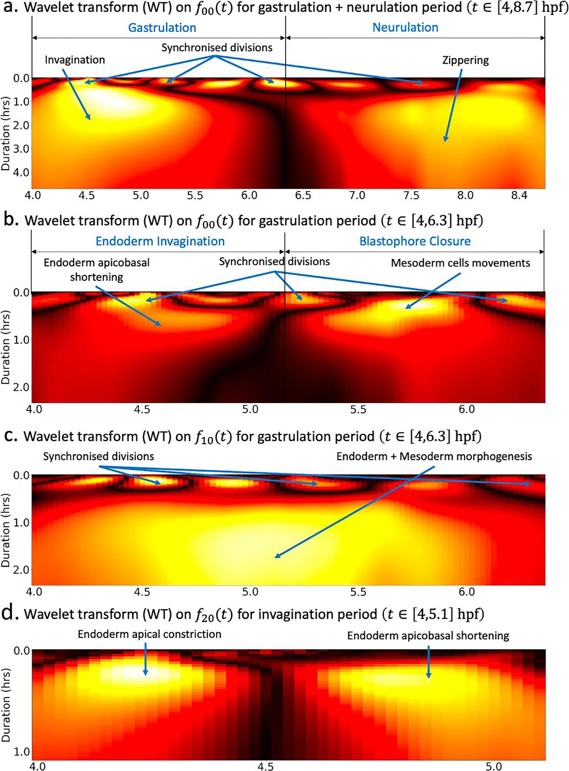
Wavelet analysis highlights multi-timescale modes of morphogenesis.
(a) Scalogram resulting from the Ricker wavelet transform applied to over the whole period covered by the dataset hpf. (b) Scalogram resulting from the Ricker wavelet transform applied to restricted to the gastrulation period hpf. The high-frequency events highlighted here represent time points of synchronized division across the embryo. The dark band in the middle separating two large red regions indicates that there are two phases of invagination characterized by large deformations and a relatively calm transition phase in between. (c) Scalogram resulting from the Ricker wavelet transform applied to restricted to the gastrulation period hpf. Similar to (b), the high-frequency events indicate synchronized division in the embryo. (d) Scalogram resulting from the Ricker wavelet transform applied to restricted to endoderm invagination hpf.
Figure 5
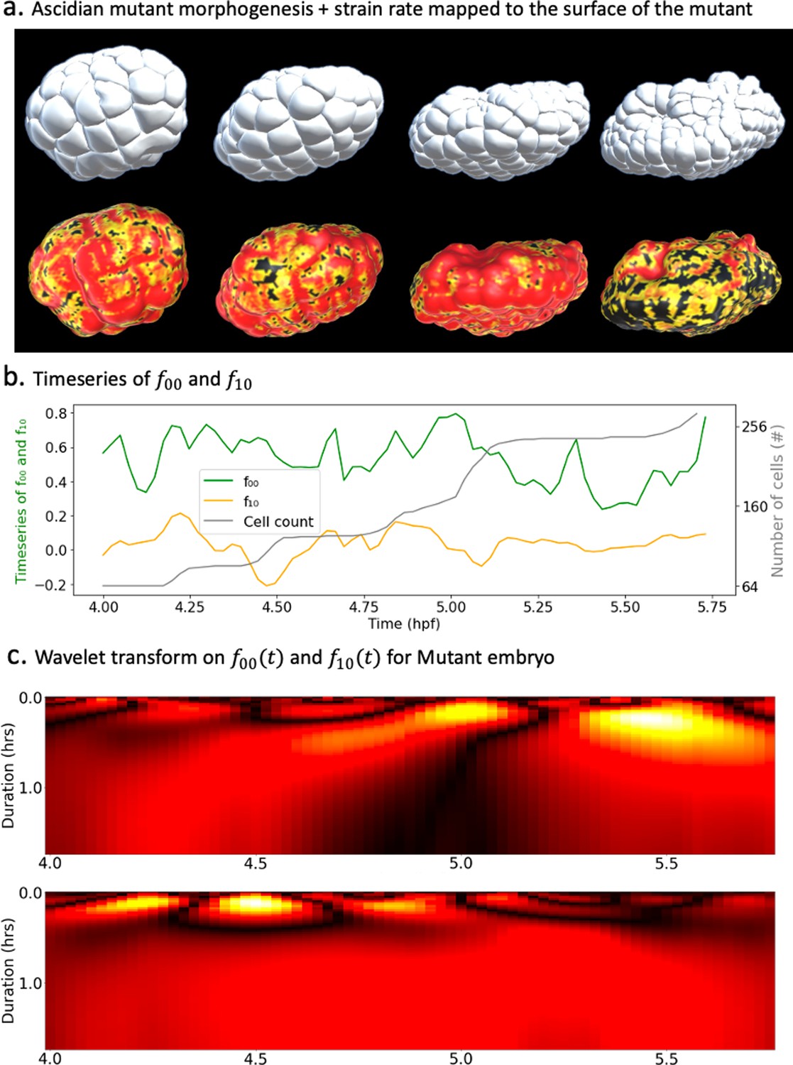
Spectral decomposition of morphogenesis in mutant embryo.
(a) Top: ascidian mutant morphogenesis. Bottom: spatiotemporal scalar strain rate field mapped to the mutant surface. (b) Time evolution of the coefficients and associated with spherical harmonics ( and ). The cell population dynamic is also included in the plot for clarity. (c) Wavelet transform applied on (top) and (bottom).
Appendix 1—figure 1
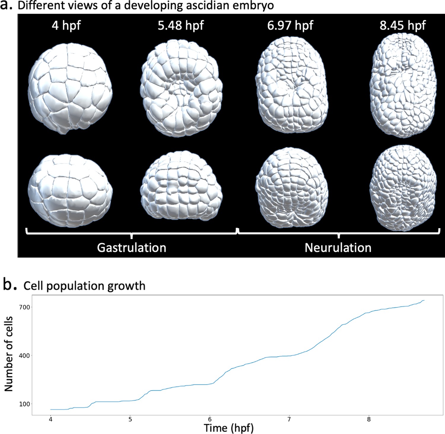
Ascidian early development gastrulation.
Tthe early ascidian embryo goes through the phases of gastrulation and neurulation. (a) Timelines of gastrulation and neurulation in a developing ascidian embryo. (b) Cell population dynamics.
Appendix 1—figure 2
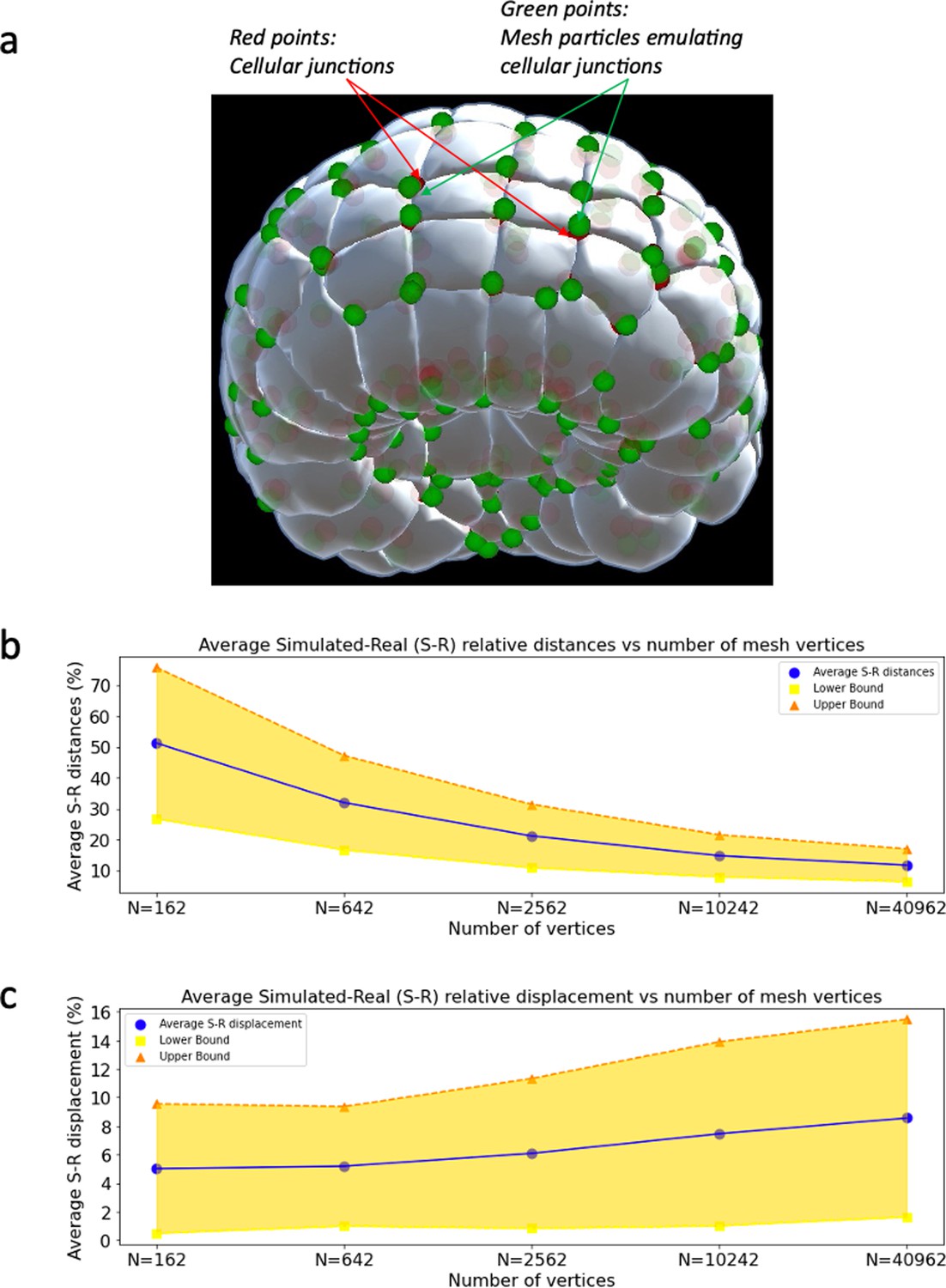
Level set scheme.
(a) Real cell junctions (red) and simulated cell junctions (green) mapped unto the embryo. (b) Average relative distances between real and simulated cell junctions as a function of number of mesh vertices. The distances are normalized by the average side length of cell apices. (c) Average relative displacement between real and simulated cell junctions as a function of number of mesh vertices.
Appendix 1—figure 3
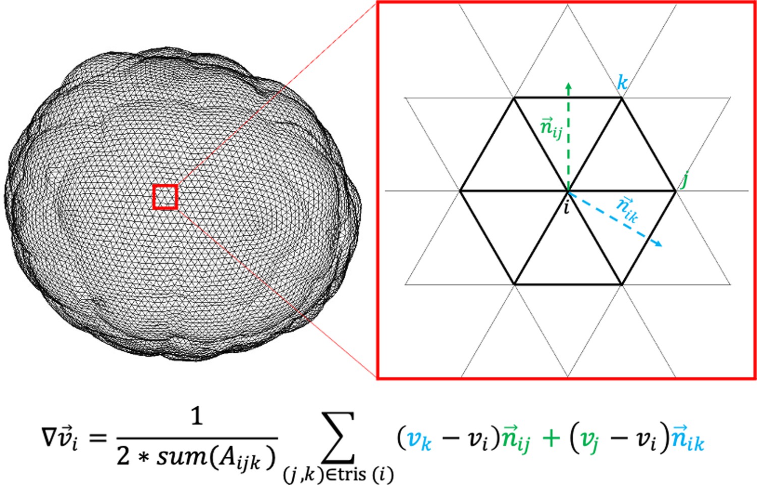
Discrete gradient computation.
Appendix 1—figure 4
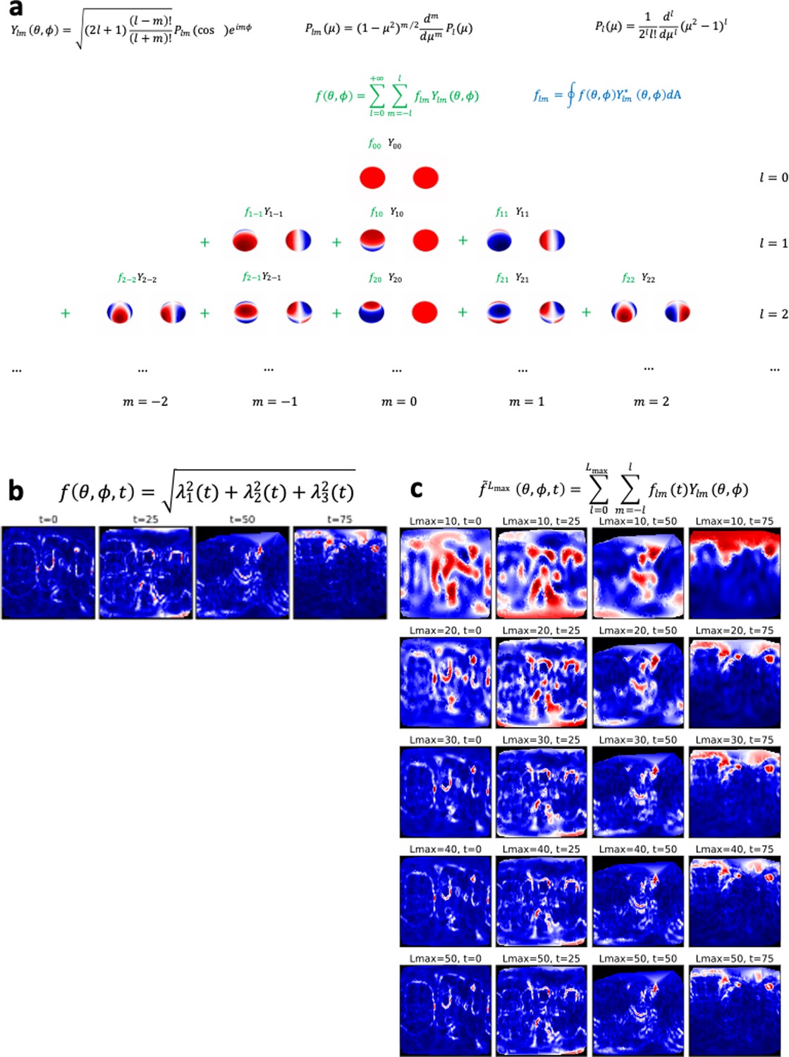
Spherical harmonics.
(a) Analytical expression and spatial representation of spherical harmonics. (b) 2D representation of the scalar strain rate field. (c) Reconstructed scalar strain rate field based on the spherical harmonics decomposition up to a degree .
Appendix 1—figure 5
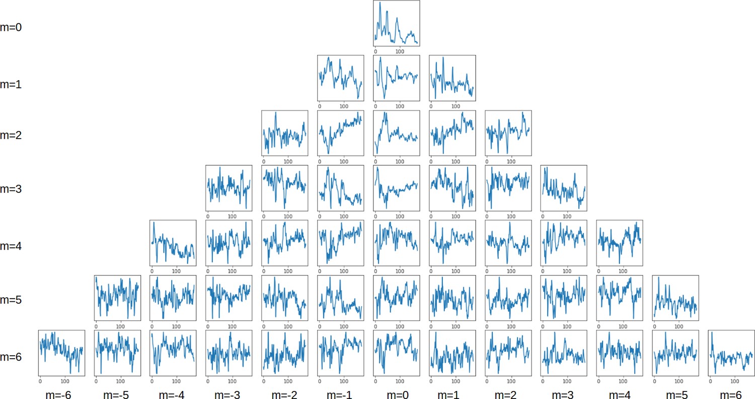
Spherical harmonics decomposition.
Time series of the spherical harmonics coefficients up to l=6.
Appendix 1—figure 6
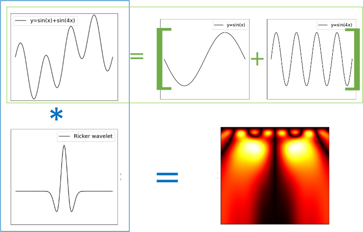
Wavelet transform.
Ricker wavelet transform of a composed signal . The transform decomposes the signal into its canonical constituents: small yellow blobs for and large yellow blobs for .
Appendix 1—figure 7
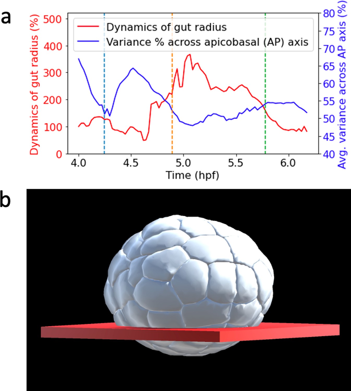
Endoderm dynamics.
(a) Spatial region of point cloud used to observe gut radius dynamics. (b) Plot of different endoderm dynamics. Blue plot: average variance of endoderm cells material particle positions across apicabasal axis during gastrulation. Red plot: dynamics of endoderm gut radius.
Additional files
Download links
A two-part list of links to download the article, or parts of the article, in various formats.
Downloads (link to download the article as PDF)
Open citations (links to open the citations from this article in various online reference manager services)
Cite this article (links to download the citations from this article in formats compatible with various reference manager tools)
Spectral decomposition unlocks ascidian morphogenesis
eLife 13:RP94391.
https://doi.org/10.7554/eLife.94391.3


