Effects of noise and metabolic cost on cortical task representations
Figures
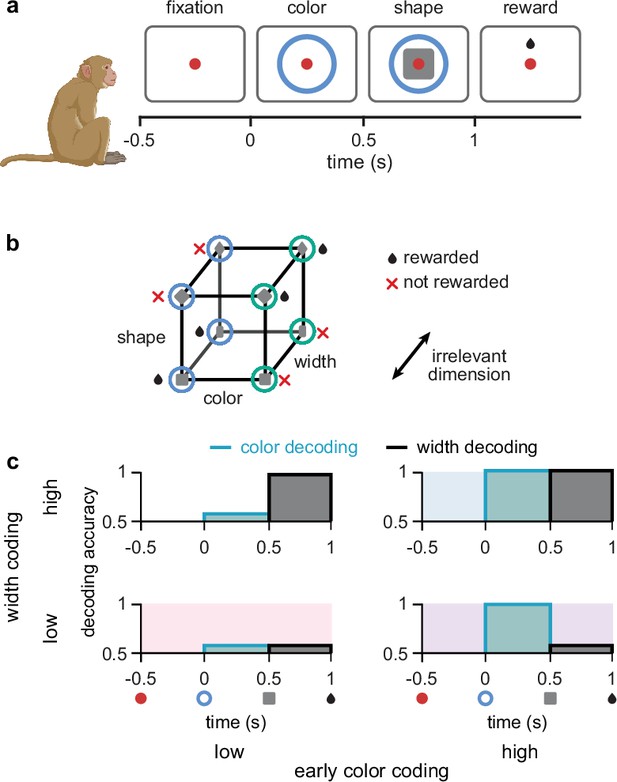
Task design and irrelevant stimulus representations.
(a) Illustration of the timeline of task events in a trial with the corresponding displays and names of task periods. Red dot shows fixation ring, blue (or green) circles appear during the color and shape periods, gray squares (or diamonds) appear during the shape period, and a juice reward is given during the reward period for rewarded combinations of color and shape stimuli (see panel b). No behavioral response was required for the monkeys as it was a passive object–association task (Wójcik, 2023). (b) Schematic showing that rewarded conditions of color and shape stimuli follows an XOR structure. In addition, the width of the shape was not predictive of reward and was thus an irrelevant stimulus dimension. (c) Schematic of four possible representational strategies, as indicated by linear decoding of population activity, for the task shown in panels a and b. Turquoise lines with shading show early color decoding and black lines with shading show width decoding. Strategies are split according to whether early color decoding is low (left column) or high (right column), and whether width decoding is low (bottom row) or high (top row).
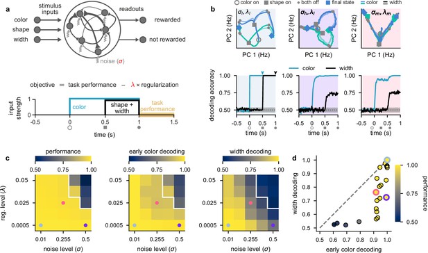
Stronger levels of noise and firing rate regularization lead to suppression of task-irrelevant stimuli in optimized recurrent networks.
(a) Top: illustration of a recurrent neural network model where each neuron receives independent white noise input with strength σ (middle). Color, shape, and width inputs are delivered to the network via three input channels (left). Firing rate activity is read out into two readout channels (either rewarded or not rewarded; right). All recurrent weights in the network, as well as weights associated with the input and readout channels, were optimized (Neural network models). Bottom: cost function used for training the recurrent neural networks (Equation 4) and timeline of task events within a trial for the recurrent neural networks (Figure 1a). Yellow shading on time axis shows the time period in which the task performance term enters the cost function (Equation 4). (b) Top: neural firing rate trajectories in the top two PCs for an example network over the course of a trial (from color stimulus onset) for a particular noise (σ) and regularization (λ) regime. Open gray circles indicate color onset, filled gray squares indicate shape onset, filled gray circles indicate offset of both stimuli, and colored thick and thin squares and diamonds indicate the end of the trial at 1.5 s for all stimulus conditions. Pale and brightly colored trajectories indicate the two width conditions. We show results for networks exposed to low noise and low regularization (; left, pale blue shading), high noise and low regularization (; middle, purple shading), and medium noise and medium regularization (; right, pink shading). Bottom: performance of a linear decoder (mean over 10 networks) trained at each time point within the trial to decode color (turquoise) or width (black) from neural firing rate activity for each noise and regularization regime. Dotted gray lines and shading show mean ± 2 s.d. of chance level decoding based on shuffling trial labels 100 times. (c) Left: performance of optimized networks determined as the mean performance over all trained networks during the reward period (a, bottom; yellow shading) for all noise (σ, horizontal axis) and regularization levels (λ, vertical axis) used during training. Pale blue, pink, and purple dots indicate parameter values that correspond to the dynamical regimes shown in panel b and Figure 1c with the same background coloring. For parameter values above the white line, networks achieved a mean performance of less than 0.95. Middle: early color decoding determined as mean color decoding over all trained networks at the end of the color period (b, bottom left, turquoise arrow) using the same plotting scheme as the left panel. Right: width decoding determined as mean width decoding over all trained networks at the end of the shape period (b, bottom left, black arrow) using the same plotting scheme as the left panel. (d) Width decoding plotted against early color decoding for all noise and regularization levels and colored according to performance. Pale blue, pink, and purple highlights indicate the parameter values shown with the same colors in panel c.
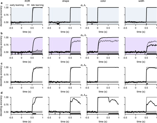
Temporal decoding for networks with different noise and regularization levels.
(a) Performance of a linear decoder trained at each time point to predict either XOR (far left), shape (middle left), color (middle right), or width (far right) from neural population activity from optimized recurrent neural networks trained in the regime. We show decoding results separately from the first half of sessions (gray, ‘early learning’) and the second half of sessions (black, ‘late learning’). Dotted gray lines and shading show mean ± 2 s.d. of chance level decoding based on shuffling trial labels 100 times. Horizontal black bars show significant differences between early and late decoding using a two-sided cluster-based permutation test and a significance threshold of 0.05 (Statistics). (b) Same as panel a, but for networks optimized in the regime. (c) Same as panel a, but for networks optimized in the regime. (d) Same as panel a, but for networks optimized in a very high regularization regime () while still being able to perform the task to a high accuracy.
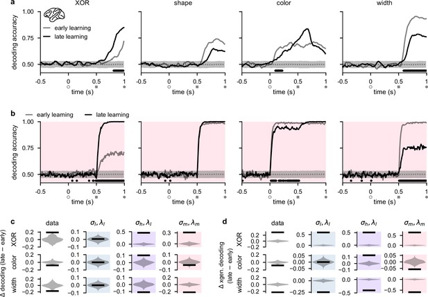
Stimulus representations in primate lateral prefrontal cortex (lPFC) correspond to a minimal representational strategy.
(a) Performance of a linear decoder trained at each time point to predict either XOR (far left), shape (middle left), color (middle right), or width (far right) from neural population activity in lPFC (Experimental materials and methods and Linear decoding). We show decoding results separately from the first half of sessions (gray, ‘early learning’) and the second half of sessions (black, ‘late learning’). Dotted gray lines and shading show mean ± 2 s.d. of chance level decoding based on shuffling trial labels 100 times. Horizontal black bars show significant differences between early and late decoding using a two-sided cluster-based permutation test and a significance threshold of 0.05 (Statistics). Open gray circles, filled gray squares, and filled gray circles on the horizontal indicate color onset, shape onset, and offset of both stimuli, respectively. (b) Same as panel a but for decoders trained on neural activity from optimized recurrent neural networks in the regime (Figure 2b–d, pink). (c) Black horizontal lines show the mean change between early and late decoding during time periods when there were significant differences between early and late decoding in the data (horizontal black bars in panel a) for XOR (top row), color (middle row), and width (bottom row). (No significant differences in shape decoding were observed in the data; cf. panel a.) Violin plots show chance differences between early and late decoding based on shuffling trial labels 100 times. We show results for the data (far left column), networks (middle left column, pale blue shading), networks (middle right column, purple shading), and networks (far right column, pink shading). (d) Same as panel c but we show results using cross-generalized decoding (Bernardi et al., 2020) during the same time periods as those used in panel c (Linear decoding).
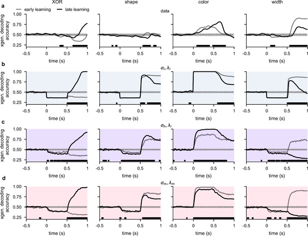
Cross-generalized temporal decoding for lateral prefrontal cortex (lPFC) recordings and networks with different noise and regularization levels.
(a) Performance of a cross-generalized decoder (Linear decoding) trained at each time point to predict either XOR (far left), shape (middle left), color (middle right), or width (far right) from neural population activity from our lPFC recordings. We show decoding results separately from the first half of sessions (gray, ‘early learning’) and the second half of sessions (black, ‘late learning’). Dotted gray lines and shading show mean ± 2 s.d. of chance level decoding based on shuffling trial labels 100 times. Horizontal black bars show significant differences between early and late decoding using a two-sided cluster-based permutation test and a significance threshold of 0.05 (Statistics). (b) Same as panel a, but for recurrent neural networks optimized in the regime. (c) Same as panel a, but for recurrent neural networks optimized in the regime. (d) Same as panel a, but for recurrent neural networks optimized in the regime.
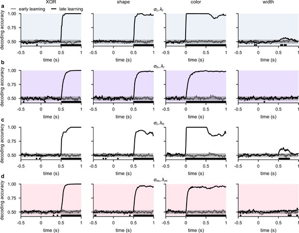
Temporal decoding for networks with input weights initialized to 0 prior to optimization.
(a) Performance of a linear decoder trained at each time point to predict either XOR (far left), shape (middle left), color (middle right), or width (far right) from neural population activity from optimized recurrent neural networks trained in the regime with input weights initialized to 0 prior to optimization (Figure 3a and b; Network optimization). We show decoding results separately from the first half of sessions (gray, ‘early learning’) and the second half of sessions (black, ‘late learning’). Dotted gray lines and shading show mean ± 2 s.d. of chance level decoding based on shuffling trial labels 100 times. Horizontal black bars show significant differences between early and late decoding using a two-sided cluster-based permutation test and a significance threshold of 0.05 (Statistics). (b) Same as panel a, but for networks optimized in the regime. (c) Same as panel a, but for networks optimized in the regime. (d) Same as panel a, but for networks optimized in the regime.
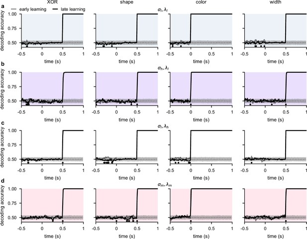
Temporal decoding for networks with input weights initialized to large random values prior to optimization.
(a) Performance of a linear decoder trained at each time point to predict either XOR (far left), shape (middle left), color (middle right), or width (far right) from neural population activity from optimized recurrent neural networks trained in the regime with input weights initialized to large random values prior to optimization (Figure 3a and b; Network optimization). We show decoding results separately from the first half of sessions (gray, ‘early learning’) and the second half of sessions (black, ‘late learning’). Dotted gray lines and shading show mean ± 2 s.d. of chance level decoding based on shuffling trial labels 100 times. Horizontal black bars show significant differences between early and late decoding using a two-sided cluster-based permutation test and a significance threshold of 0.05 (Statistics). (b) Same as panel a, but for networks optimized in the regime. (c) Same as panel a, but for networks optimized in the regime. (d) Same as panel a, but for networks optimized in the regime.
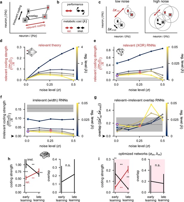
Theoretical predictions for strength of relevant and irrelevant stimulus coding and comparison to lateral prefrontal cortex (lPFC) recordings.
(a) Schematic of activity in neural state space for two neurons for a task involving two relevant (black drops vs. red crosses) and two irrelevant stimuli (thick vs. thin squares). Strengths of relevant and irrelevant stimulus coding are shown with red and black arrows, respectively, and the overlap between relevant and irrelevant coding is also shown (‘overlap’). (b) Schematic of our theoretical predictions for the optimal setting of relevant (red arrows) and irrelevant (black arrows) coding strengths when either maximizing performance (top) or minimizing a metabolic cost with strength λ (bottom; see Equation 4). (c) Schematic of our theoretical predictions for the strength of relevant (; black drops vs. red crosses; red arrows) and irrelevant (; thick vs. thin squares; black arrows) coding when jointly optimizing for both performance and a metabolic cost (cf. panel b). In the low noise regime (left), relevant conditions are highly distinguishable and irrelevant conditions are poorly distinguishable as well as strongly orthogonal to the relevant conditions. In the high noise regime (right), all conditions are poorly distinguishable. (d) Our theoretical predictions (Equation S34) for the strength of relevant coding (, see panel c) as a function of the noise level σ (horizontal axis) and firing rate regularization strength λ (colorbar). (e) Same as panel d but for our optimized recurrent neural networks (Figure 2) where we show the strength of relevant (XOR) coding (Measuring stimulus coding strength). Pale blue, purple, and pink highlights correspond to the noise and regularization strengths shown in Figure 2c and d. Gray dotted line and shading shows mean ±2 s.d. (over 250 networks; 10 networks for each of the 25 different noise and regularization levels) of prior to training. (f) Same as panel e but for the strength of irrelevant (width) coding (). The black arrow indicates the theoretical prediction of 0 irrelevant coding. (g) The absolute value of the normalized dot product (overlap) between relevant and irrelevant representations (, i.e. 0 implies perfect orthogonality and 1 implies perfect overlap) for our optimized recurrent neural networks. The black arrow indicates the theoretical prediction of 0 overlap. (h) Left: coding strength (length of arrows in panel a; Measuring stimulus coding strength) for relevant (XOR; red) and irrelevant (width; black) stimuli during early and late learning for our lPFC recordings. Right: the absolute value of the overlap between relevant and irrelevant representations for our lPFC recordings (0 implies perfect orthogonality and 1 implies perfect overlap). Error bars show the mean ± 2 s.d. over 10 non-overlapping splits of the data. (i) Same as panel h but for the optimized recurrent neural networks in the regime (see pink dots in Figure 2). Error bars show the mean ± 2 s.d. over 10 different networks. p-Values resulted from a two-sided Mann–Whitney U test (*, p<0.05; **, p<0.01; n.s., not significant; see Statistics).
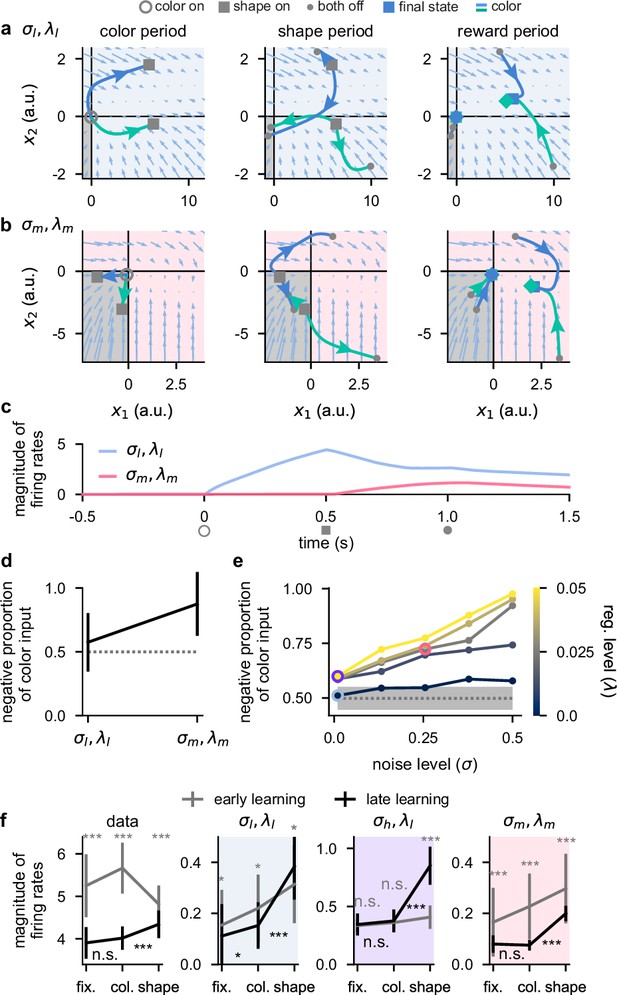
Activity-silent, sub-threshold dynamics lead to the suppression of dynamically irrelevant stimuli.
(a) Sub-threshold neural activity ( in Equation 1) in the full state space of an example two-neuron network over the course of a trial (from color onset) trained in the regime. Pale blue arrows show flow field dynamics (direction and magnitude of movement in the state space as a function of the momentary state). Open gray circles indicate color onset, gray squares indicate shape onset, filled gray circles indicate offset of both stimuli, and colored squares and diamonds indicate the end of the trial at 1.5 s. We plot activity separately for the three periods of the task (color period, left; shape period, middle; reward period, right). We plot dynamics without noise for visual clarity. (b) Same as panel a but for a network trained in the regime. (c) Momentary magnitude of firing rates (; i.e. momentary metabolic cost, see Equation 4) for the two-neuron networks from panels a (blue line) and b (pink line). (d) Mean ± 2 s.d. (over 10 two-neuron networks) proportion of color inputs that have a negative sign for the two noise and regularization regimes shown in panels a–c. Gray dotted line shows chance level proportion of negative color input. (e) Mean (over 10 fifty-neuron networks) proportion of color inputs that have a negative sign for all noise (horizontal axis) and regularization (colorbar) strengths shown in Figure 2c and d. Pale blue, purple, and pink highlights correspond to the noise and regularization strengths shown in Figure 2c and d. Gray dotted line and shading shows mean ± 2 s.d. (over 250 networks; 10 networks for each of the 25 different noise and regularization levels) of the proportion of negative color input prior to training (i.e. the proportion of negative color input expected when inputs are drawn randomly from a Gaussian distribution; Network optimization). (f) Momentary magnitude of firing rates () for our lateral prefrontal cortex (lPFC) recordings (far left) and 50-neuron networks in the regime (middle left, blue shading), regime (middle right, purple shading), and regime (far right, pink shading). Error bars show the mean ± 2 s.d. over either 10 non-overlapping data splits for the data or over 10 different networks for the models. p-Values resulted from a two-sided Mann–Whitney U test (*, p<0.05; **, p<0.01; ***, p<0.001; n.s., not significant; see Statistics).
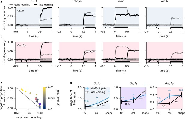
Temporal decoding for two-neuron networks and supplemental analysis of suppression of dynamically irrelevant stimuli.
(a) Performance of a linear decoder trained at each time point to predict either XOR (far left), shape (middle left), color (middle right), or width (far right) from neural population activity from optimized two-neuron networks (Figure 5a–d) trained in the regime. Dotted gray lines and shading show mean ± 2 s.d. of chance level decoding based on shuffling trial labels 100 times. Horizontal black bars show significant differences between early and late decoding using a two-sided cluster-based permutation test and a significance threshold of 0.05 (Statistics). (b) Same as panel a but for two-neuron networks trained in the regime. (c) Mean (over 10 fifty-neuron networks) proportion of color inputs that have a negative sign for all noise and regularization strengths (colorbar) plotted against early color decoding (see Figure 2c, middle). Pale blue, purple, and pink highlights correspond to the noise and regularization strengths shown in Figure 2c. Gray dotted line shows the negative identity line shifted to intercept the vertical axis at 1. (d) Momentary magnitude of firing rates (; i.e. momentary metabolic cost, see Equation 4) for 50-neuron networks in the regime (left, blue shading), regime (purple shading), and regime (right, pink shading). We show results after learning (black lines, ‘late learning’; repeated from Figure 5f) and when shuffling color, shape, and width input weights (blue lines, ‘shuffle inputs’; Measuring the magnitude of neural firing rates). Error bars show the mean ± 2 s.d. over 10 different networks. p-Values resulted from a two-sided Mann–Whitney U test (*, p<0.05; **, p<0.01; ***, p<0.001; n.s., not significant; see Statistics).
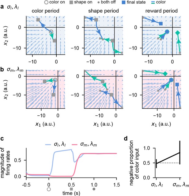
Activity-silent, sub-threshold dynamics lead to the suppression of dynamically irrelevant stimuli in networks with a sigmoid nonlinearity.
(a) Sub-threshold neural activity ( in Equation 1) in the full state space of an example two-neuron network with a sigmoid () nonlinearity over the course of a trial (from color onset) trained in the regime (Neural network models). Pale blue arrows show flow field dynamics (direction and magnitude of movement in the state space as a function of the momentary state). Open gray circles indicate color onset, gray squares indicate shape onset, filled gray circles indicate offset of both stimuli, and colored squares and diamonds indicate the end of the trial at 1.5 s. We plot activity separately for the three periods of the task (color period, left; shape period, middle; reward period, right). We plot dynamics without noise for visual clarity. (b) Same as panel a but for a network trained in the regime. (c) Momentary magnitude of firing rates (; i.e. momentary metabolic cost, see Equation 4) for the two-neuron networks from panels a (blue line) and b (pink line). (d) Mean ± 2 s.d. (over 10 two-neuron networks) proportion of color inputs that have a negative sign for the two noise and regularization regimes shown in panels a–c. Gray dotted line shows chance level proportion of negative color input.
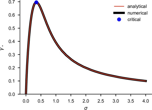
Plot of as a function of σ obtained by numerically optimizing Equation S30 (black), or using the analytical expression in Equation S34 (red).
Blue dot shows (analytically computed) critical values where has a maximum (Equations S36 and S37). We used λ=1 for these results.
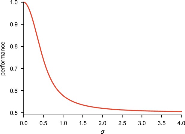
Plot of as a function of σ when using that is optimized as in Appendix 1—figure 1 (Equation S38).
We used λ=1 for these results. All other parameters were optimized in all cases.
Tables
Parameters used in the simulations of our models.
| Symbol | Figures 2 and 3b-dFigure 4e-g,i, Figure 5e,f Figure 2—figure supplement 1a-c, Figure 3—figure supplements 2 and 3, Figure 3—figure supplement 1b,c, and Figure 5—figure supplement 1c,d | Figure 5a-d and Figure 5—figure supplement 1a,b | Figure 5—figure supplement 2 | Figure 2—figure supplement 1d | Units | Description |
|---|---|---|---|---|---|---|
| N | 50 | 2 | 2 | 50 | - | number of neurons |
| t0 | –0.5 | –0.5 | –0.5 | –0.5 | s | simulation start time |
| 1.5 | 1.5 | 1.5 | 1.5 | s | simulation end time | |
| τ | 0.05 | 0.05 | 0.05 | 0.05 | s | effective time constant |
| ReLU | ReLU | ReLU | Hz | nonlinearity | ||
| σ | variable* | [0.01, 0.255] | [0.01, 0.255] | 0.01 | - | noise standard deviation |
| λ | variable† | [0.0005, 0.02525] | [0.0005, 0.02525] | 0.5 | s | regularization strength |
| optimized ‡ | optimized ‡ | optimized ‡ | optimized ‡ | s | weight matrix | |
| optimized ‡ | optimized ‡ | optimized ‡ | optimized ‡ | - | color input weights | |
| optimized ‡ | optimized ‡ | optimized ‡ | optimized ‡ | - | shape input weights | |
| optimized ‡ | optimized ‡ | optimized ‡ | optimized ‡ | - | width input weights | |
| optimized ‡ | optimized ‡ | optimized ‡ | optimized ‡ | - | bias | |
| optimized ‡ | optimized ‡ | optimized ‡ | optimized ‡ | s | readout weights | |
| optimized ‡ | optimized ‡ | optimized ‡ | optimized ‡ | - | readout bias |


