Sensory-memory interactions via modular structure explain errors in visual working memory

Abstract
eLife assessment
Introduction
Results
Discussion
Methods
Data availability
References
Article and author information
Metrics

Abstract

Errors in stimulus estimation reveal how stimulus representation changes during cognitive processes. Repulsive bias and minimum variance observed near cardinal axes are well-known error patterns typically associated with visual orientation perception. Recent experiments suggest that these errors continuously evolve during working memory, posing a challenge that neither static sensory models nor traditional memory models can address. Here, we demonstrate that these evolving errors, maintaining characteristic shapes, require network interaction between two distinct modules. Each module fulfills efficient sensory encoding and memory maintenance, which cannot be achieved simultaneously in a single-module network. The sensory module exhibits heterogeneous tuning with strong inhibitory modulation reflecting natural orientation statistics. While the memory module, operating alone, supports homogeneous representation via continuous attractor dynamics, the fully connected network forms discrete attractors with moderate drift speed and nonuniform diffusion processes. Together, our work underscores the significance of sensory-memory interaction in continuously shaping stimulus representation during working memory.

eLife assessment

This important computational study provides new insights into how neural dynamics may lead to time-evolving behavioral errors as observed in certain working-memory tasks. By combining ideas from efficient coding and attractor neural networks, the authors construct a two-module network model to capture the sensory-memory interactions and the distributed nature of working memory representations. They provide convincing evidence supporting that their two-module network, although none of the alternative circuit structures they considered can account for error patterns reported in orientation-estimation tasks with delays.

https://doi.org/10.7554/eLife.95160.4.sa0

Significance of the findings:

Important: Findings that have theoretical or practical implications beyond a single subfield

Landmark
Fundamental
Important
Valuable
Useful

Strength of evidence:

Convincing: Appropriate and validated methodology in line with current state-of-the-art

Exceptional
Compelling
Convincing
Solid
Incomplete
Inadequate

During the peer-review process the editor and reviewers write an eLife Assessment that summarises the significance of the findings reported in the article (on a scale ranging from landmark to useful) and the strength of the evidence (on a scale ranging from exceptional to inadequate). Learn more about eLife Assessments

Introduction

The brain does not faithfully represent external stimuli. Even for low-level features like orientation, spatial frequency, or color of visual stimuli, their internal representations are thought to be modified by a range of cognitive processes, including perception, memory, and decision (Geisler, 2008; Webster, 2015; Bays et al., 2022). Experimental studies quantified such modification by analyzing behavior data or decoding neural activities. For instance, biases of errors, the systematic deviation from the original stimuli, observed in estimation tasks have been used as indirect evidence to infer changes in the internal representations of stimuli (Wei and Stocker, 2017).

One important source of biases is adaptation to environmental statistics, such as the nonuniform stimulus distribution found in nature or the limited range in specific settings. Cardinal repulsion, which refers to the systematic shift away from the horizontal and vertical orientations observed in many perceptual tasks, is one of the examples (de Gardelle et al., 2010). Theoretical works suggest that such a bias pattern reflects the prevalence of the cardinal orientations in natural scenes (Girshick et al., 2011). Similarly, the variance of errors for orientation stimuli was found to be inversely proportional to the stimulus statistics, minimum at cardinal and maximum at oblique orientations (van Bergen et al., 2015). It was postulated that the dependence of biases and variance of errors on natural statistics results from sensory encoding optimized to enhance precision around the most common stimuli (Ganguli and Simoncelli, 2014; Wei and Stocker, 2015; Wei and Stocker, 2017).

On the other hand, there is a growing body of evidence indicating that error patterns are not solely influenced by sensory encoding but are also shaped by memory processes. In delayed estimation tasks, where participants are presented with stimuli followed by a delay period during which they rely on their working memory for estimation, it has been observed that representations of orientation or color stimuli undergo gradual and continuous modifications throughout the delay period (Panichello et al., 2019; Bae, 2021; Gu et al., 2023). Such dynamic error patterns are inconsistent with sensory encoding models, most of which only establish a static relationship between stimuli and internal representations.

Traditional working memory models are not suitable either. Most of them are constructed to faithfully maintain information about stimuli during the delay period, and thus, the memory representation has a similar geometry as that of the stimuli (Wang, 2001; Khona and Fiete, 2022). For continuous stimuli such as orientation, location, direction, or color, all stimuli are equally maintained in ring-like memory activities, predicting no biases (Zhang, 1996; Compte et al., 2000; Burak and Fiete, 2009).

How can we explain error patterns in working memory tasks that are similar to those observed in perception tasks? Here, we claim that not a single-module but a two-module network with recursive interaction is required. Each module has a distinct role – sensory encoding and memory maintenance. To illustrate this, we use orientation stimuli and examine how their representations change during the delayed estimation tasks. We employ two approaches to find solutions for generating correct error patterns. The first extends previously suggested sensory encoding models, while the second modifies low-dimensional memory models based on attractor dynamics. These approaches are integrated into the network models, which link network connectivity to neuronal tuning properties and behavioral error patterns and reveal the attractor dynamics through low-dimensional projection. Our results show that the sensory-memory interacting networks outperform single-module networks with better control over the shapes and evolution of dynamic error patterns. Furthermore, our network models emphasize the importance of inhibitory tuning in sensory circuits for generating correct error patterns under typical associative learning of natural statistics. Finally, we provide testable predictions regarding the effect of perturbations in sensory-memory interactions on error patterns in delayed estimation tasks.

Results

Low-dimensional attractor models

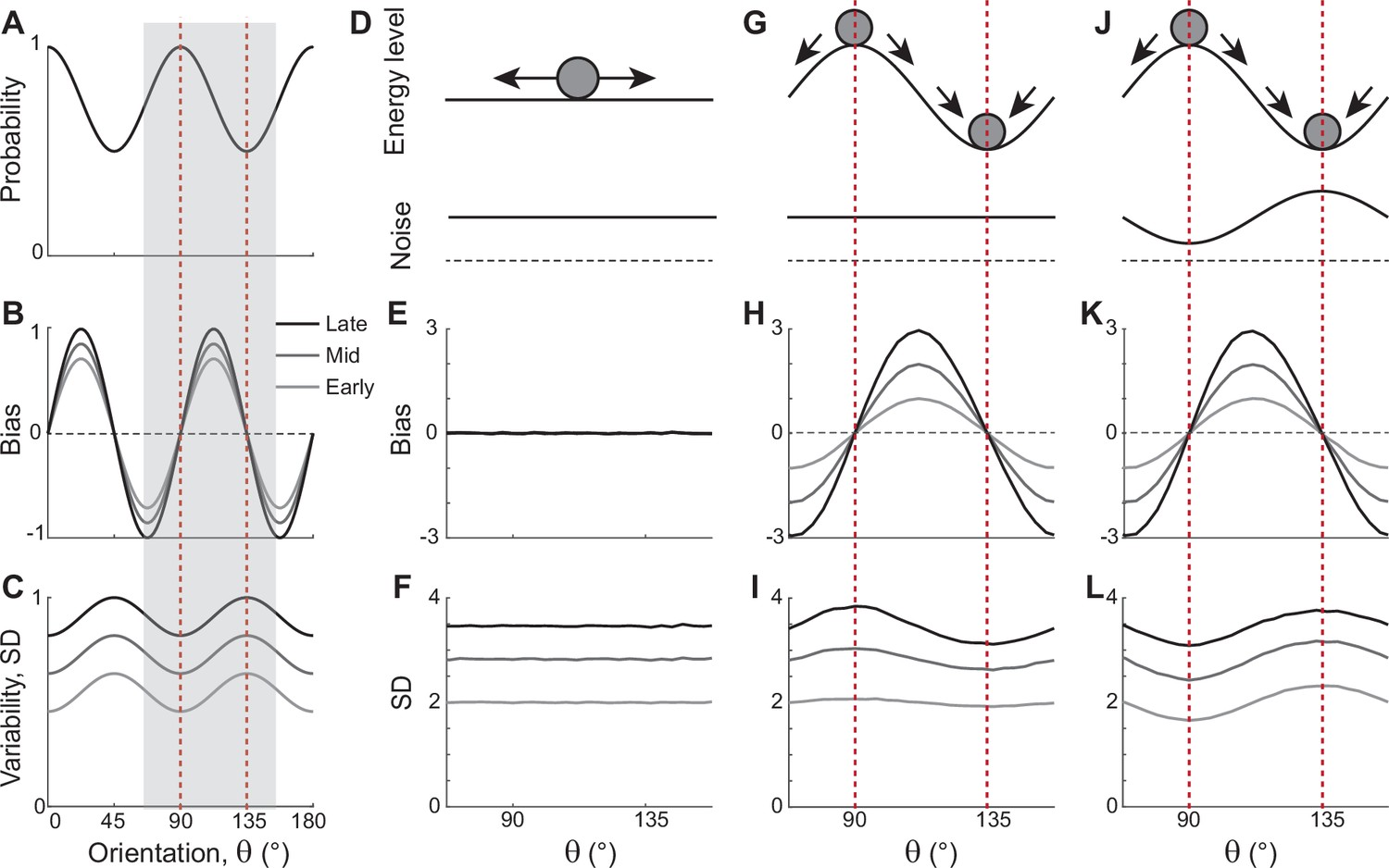
In natural images, cardinal orientations are the most prevalent (Figure 1A). Error patterns in estimation tasks show dependence on such natural statistics, such as biases away from cardinal orientations where the variance of errors is nonetheless minimal (Figure 1B and C). In delayed estimation tasks, such a bias pattern is consolidated in time (Figure 1B). Also, experimental data suggested that estimation errors increase with a longer delay (Wimmer et al., 2014; Schneegans and Bays, 2018), while the precision is still highest at cardinal orientations (van den Berg et al., 2012; Bays, 2014; van Bergen et al., 2015). Thus, we assumed that the variance of errors increases as keeping its characteristic shape (Figure 1C). To explain these errors across orientations and over time, we first explored the underlying working memory mechanism. We considered low-dimensional attractor models with input noise that describe the drift and diffusion of the memory states. Here, we show that two prominent classes of previously suggested models are inconsistent with experimental observations and examine what modification to the models is required.

Figure 1

Download asset Open asset

Error patterns of orientation stimuli in delayed estimation tasks and low-dimensional attractor models.

(**A–C**) Characteristic patterns of natural statistics of orientation stimuli $θ$ (A), bias (B), and standard deviation (SD; C) during the delay period observed experimentally. Cardinal orientations are predominant in natural images (A). Bias and SD increase during the delay period, keeping patterns of repulsive bias (B) and minimum variance (C) around cardinal orientations. These characteristic patterns are visualized using trigonometric functions, and the range is normalized by their maximum values. Red vertical lines correspond to representative cardinal and oblique orientations, and with a periodicity of the error patterns, we only show the gray-shaded range in the remaining panels. (**D–L**) Comparison of different attractor models. (**D–F**) Continuous attractors with constant noise. Energy potential is flat (D), resulting in no bias (E) and uniform SD with uniform noise (F). (**G–L**) Discrete attractors with constant (**G–I**) and nonuniform noise (**J–L**). The discrete attractor models have potential hills and wells at cardinal and oblique orientations, respectively (**G, J**). While the bias patterns depend only on the energy landscape (**H, K**), SD representing variability also depends on noise (**I, L**). For the correct SD pattern (L), uneven noise with its maxima at the obliques (J) is required. Bias and SD patterns in the attractor models were obtained by running one-dimensional drift-diffusion models (see Methods).

The most widely accepted model for working memory of orientation stimuli has continuous attractor dynamics, which assumes that all orientations are equally encoded and maintained (Figure 1D–F). Each attractor corresponds to the memory state for different stimuli and forms a continuous ring following the geometry of orientation stimuli. The dynamics along continuous attractors are conceptually represented as movement along a flat energy landscape (Figure 1D). Without external input, there is no systematic shift of mean activity, i.e., no drift during the delay period (Figure 1E). Also, under the assumption of equal influence of noise for all orientations, the variance of errors is spatially flat with constant diffusion along the ring, while the overall magnitude increases over time due to the accumulation of noise (Figure 1F).

While such continuous attractor models have been considered suitable for memory storage of continuous stimuli, they cannot capture drift dynamics observed during the delay period. Instead, discrete attractor models with uneven energy landscapes have been suggested with the energy wells corresponding to discrete attractors (Figure 1G–I). As evolution toward a few discrete attractors creates drift dynamics, the bias increases during the delay (Figure 1H). Also, discrete attractor models naturally produce nonuniform variance patterns. Even with constant noise along the ring, variance becomes minimum/maximum at the attractors/repellers due to the drift dynamics (Figure 1I). However, discrete attractor models with constant noise yield inconsistent results when inferring the locus of attractors from the bias and variance patterns observed in the data. Cardinal orientations should be the repeller to account for cardinal repulsion. In contrast, the minimum variance observed at the cardinal orientations suggests they should be the attractors.

How can such inconsistency be resolved? One possible solution is discrete attractor models with nonuniform noise amplitude (Figure 1J). Let’s consider that attractors are formed at oblique orientations to generate correct bias patterns (Figure 1K). Additionally, we assumed that noise has the highest amplitude at the obliques. When the difference in the noise amplitude is large enough to overcome the attraction toward the obliques, the models can produce correct variance patterns, maximum at the obliques and minimum at cardinal orientations (Figure 1L). In sum, unlike two prominent memory models, continuous attractors or discrete attractors with constant noise, discrete attractors with maximum noise at the obliques could reproduce experimentally observed error patterns of orientation stimuli. Note that these attractor models often simplify the full network dynamics. Namely, the drift and diffusion terms are derived by projecting network dynamics onto low-dimensional memory states (Burak and Fiete, 2012; Darshan and Rivkind, 2022). Thus, it is still in question whether there exist memory networks that can implement attractor dynamics with correct drift and diffusion terms.

Bayesian sensory model and extension

Before exploring full memory network models, we note that previous theoretical works for sensory processing suggested that Bayesian inference with efficient coding could generate the repulsive bias and the lowest variance at cardinal orientations (Wei and Stocker, 2015; Wei and Stocker, 2017). Efficient coding theory suggests the sensory system should enhance the sensitivity around more common stimuli. For orientation stimuli, precision should be highest around cardinal directions, which could be achieved by sharpening the likelihood functions. Equipped with Bayesian optimal readout, such a sensory system could reproduce correct error patterns observed in perceptual tasks for various visual stimuli, including orientations (Figure 2).

Figure 2

Download asset Open asset

Extension of Bayesian sensory models.

(A) Schematics of extension to memory processing. We adapted the previous Bayesian models (Wei and Stocker, 2015) for sensory encoding where $θ$ and $\hat{θ}$ are the input and output of sensory modules, respectively. We added a memory module where it maintains $\hat{θ}$ with the addition of memory noise $ξ$ . The output of the memory module, $\hat{θ} + ξ$ , is fed back to the sensory module as the input for the next iteration. (B) Illustration of the first iteration of sensory-memory interaction. Prior distribution follows the natural statistics (top), resulting in a sharper likelihood function near cardinal orientations (middle). Combining prior and likelihood functions leads to the posterior distribution of decoded $\hat{θ}$ (light colors at the bottom), which is broadened with the addition of memory noise (dark colors at the bottom). Different curves correspond to different initial $θ$ . (C) Bias (top) and SD (bottom) patterns obtained from decoded $\hat{θ}$ for the first, second, and third iterations.

However, such models only account for the relationship between external and perceived stimuli during sensory processing, resulting in static error patterns. Here, we extended the framework so that the system can maintain information about the stimulus after its offset while bias and variance of errors grow in time (Figure 2A). We added a memory stage to Bayesian sensory models such that the memory stage receives the output of the sensory stage and returns it as the input after the maintenance. For instance, let’s denote the external orientation stimulus given during the stimulus period as $θ_{1}$ . The sensory stage receives $θ_{1}$ as input and generates the perceived orientation, ${\hat{θ}}_{1}$ , which varies from trial to trial with sensory noise (Figure 2B). Through the memory stage, ${\hat{θ}}_{1}$ is returned as the input to the sensory stage for the next iteration with the addition of memory noise $ξ_{1}$ .

Such a recursive process mimics interactions between sensory and memory systems where the sensory system implements efficient coding and Bayesian inference, and the memory system faithfully maintains information. As the recursive process iterates, the distribution of the internal representation of orientation broadens due to the accumulation of noise from the sensory and memory systems. This leads to an increase in bias and variance at each step while keeping their characteristic shapes (Figure 2C). Thus, recurrent interaction between sensory and memory systems during the delay period, each of which meets different demands, successfully reproduces correct error patterns observed in memory tasks.

Network models with sensory and memory modules

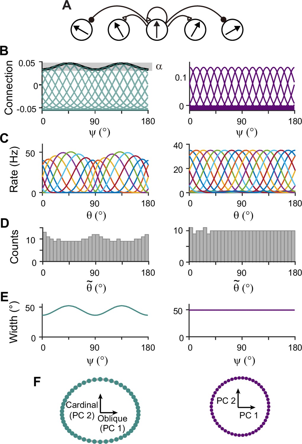
Next, we construct network models capturing the sensory-memory interactions formalized under the Bayesian framework. We consider two-module networks where each module corresponds to the sensory and memory systems. To generate orientation selectivity, both modules have a columnar architecture where neurons in each column have a similar preference for orientation (Figure 3A). However, their connectivity structures are different (Figure 3B). The memory module in isolation resembles the traditional ring attractor network with a strong and homogeneous recurrent connection. This enables the memory module in isolation to maintain information about all orientations equally during the delay period (Figure 3B–F, right). Conversely, the recurrent connectivity strengths in the sensory module are relatively weak, such that without connection to the memory module, the activities during the delay period decay back to the baseline levels (Figure 3B, left). Furthermore, the connectivity strengths across columns are heterogeneous, particularly stronger at the obliques. As a result, the tuning curves near cardinal orientations can be sharper and denser, consistent with experimental observations showing a larger number of cardinally tuned neurons (Li et al., 2003; Shen et al., 2014) and their narrower tuning (Li et al., 2003; Kreile et al., 2011; Figure 3C–F, left). Different response activities of the two modules in isolation are demonstrated in their response manifolds as more dispersed representations around cardinal orientations in the sensory module, compared to the ring-like geometry of the memory module (Figure 3F).

Figure 3

Download asset Open asset

Network models of sensory and memory circuits in isolation, implementing efficient coding and ring attractor dynamics, respectively.

(A) Schematics of columnar architecture for orientation selectivity. Neurons in the same column have similar preferred orientations, and recurrent connections are a combination of local excitation and global inhibition, represented as triangles and circles, respectively. (**B–F**) Connectivity and tuning properties of the sensory network (left column) and memory network (right column). (B) Example connectivity strengths. We indexed neurons by $ψ$ ranging uniformly from 0° to 180°. The connectivity strengths depend only on $ψ$ ’s of the presynaptic and postsynaptic neurons. Each curve shows the connectivity strengths from presynaptic neuron $ψ$ to an example postsynaptic neuron. Unlike the homogeneous connectivity in the memory network (right), the sensory connectivity is heterogeneous, and its degree is denoted by $α$ . (C) Heterogeneous tuning curves for different stimulus $θ$ in the sensory network in the stimulus period (left) and homogeneous ones in the memory network in the delay period (right). The memory network can sustain persistent activity in isolation, while the sensory network cannot. (D) Histograms of the preferred orientations. We measured the maximum of the tuning curve of each neuron, denoted as $\tilde{θ}$ (Methods). The heterogeneous sensory network has more cardinally tuned neurons. (E) Widths of tuning curves measured at the half maximum of the tuning curves (Methods). The sensory tuning curves sharpen around cardinal orientations. Each neuron is labeled with its index $ψ$ as in (B). (F) Neural manifolds projected onto the first two principal components of activities during the stimulus period (left) and during the delay period (right). The neural manifold of the sensory network resembles a curved ellipsoid, while the manifold corresponding to the homogeneous memory network is a perfect ring.

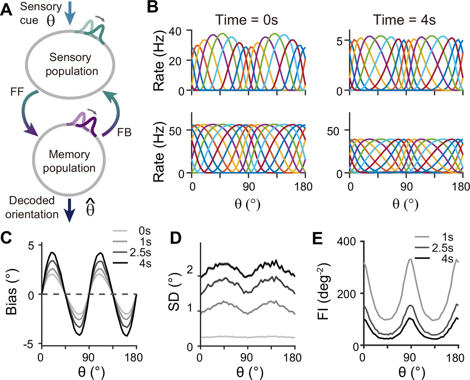
For sensory-memory interacting networks, we connected the two modules with intermodule connections set to be stronger between neurons with similar orientation selectivity (Figure 4A). Activity profiles in both modules follow that of the sensory module – heterogeneous with narrower and denser tuning curves around cardinal orientations, leading to higher sensitivity (Figure 4B). Such activity pattern is maintained even during the delay period when recurrent connections in the memory module support activities of both sensory and memory modules (Figure 4B, right). Note that while sensory activities convey stimulus information during the delay period, their overall firing rates are much lower than those during the stimulus period with weak interconnection strengths. Such low firing rates may lead to both positive and negative evidence of sustained activity in early sensory areas (Leavitt et al., 2017).

Figure 4 with 2 supplements see all

Download asset Open asset

Network model with interacting sensory and memory modules generates correct error patterns in delayed estimation tasks.

(A) Schematic of two-module architecture. The sensory and memory modules are connected via feedforward and feedback connectivity to form a closed loop. The sensory module receives external input with orientation $θ$ while internal representation is decoded from the memory module, denoted as $\hat{θ}$ . (B) Tuning curves of sensory (upper panels) and memory (lower panels) modules at the end of the stimulus epoch (i.e. the beginning of the delay epoch; left panels) and during the delay period (right panels). Note that while both modules can sustain persistent activity in the delay period, the firing rates of the sensory module are significantly lower than those in the stimulus period (upper right). (**C–E**) Bias (C), standard deviation (SD; D), and Fisher information (FI; E) patterns. Error patterns evaluated at 1, 2.5, and 4 s into the delay are consistent with the characteristic patterns observed experimentally in delayed estimation tasks (Figure 1A–C). However, the low SD right after the stimulus offset in (D) deviates from error patterns seen in perception tasks (see Discussion). While FI decays due to noise accumulation, it is largest around cardinal orientations, corresponding to a smaller discrimination threshold (E). In (C) and (D), shaded areas mark the ±s.e.m. of 1000 realizations.

When the internal representation of the orientation stimulus is read from the memory module using a population vector decoder mimicking Bayesian optimal readout (Fischer, 2010), the sensory-memory interacting network exhibits repulsive bias and minimum variance at cardinal orientations, inheriting from efficient sensory coding (Figure 4C and D). Similar error patterns were observed when decoded from activities of the sensory module (Figure 4—figure supplement 1). Such bias increases during the delay period with increasing asymmetry of tuning widths despite lower firing rates than the stimulus period (Figure 4—figure supplement 2). At the same time, errors gradually increase due to noise accumulation in time, as in typical memory networks (Compte et al., 2000; Burak and Fiete, 2012). Note that the variance of errors is negligible during stimulus presentation when the external input overwhelms internal noise, which may not fully account for the variability observed during perception tasks (see Discussion). We obtained Fisher information measuring sensitivity at each orientation from the neural responses (see Methods). Opposite to the variance of errors, Fisher information is highest at cardinal orientations, while it decreases during the delay period (Figure 4E). Thus, the sensory-memory interacting network model that mechanistically embodies the extension of the Bayesian sensory model correctly reproduces the error patterns observed in delayed estimation tasks.

Analysis of low-dimensional memory states

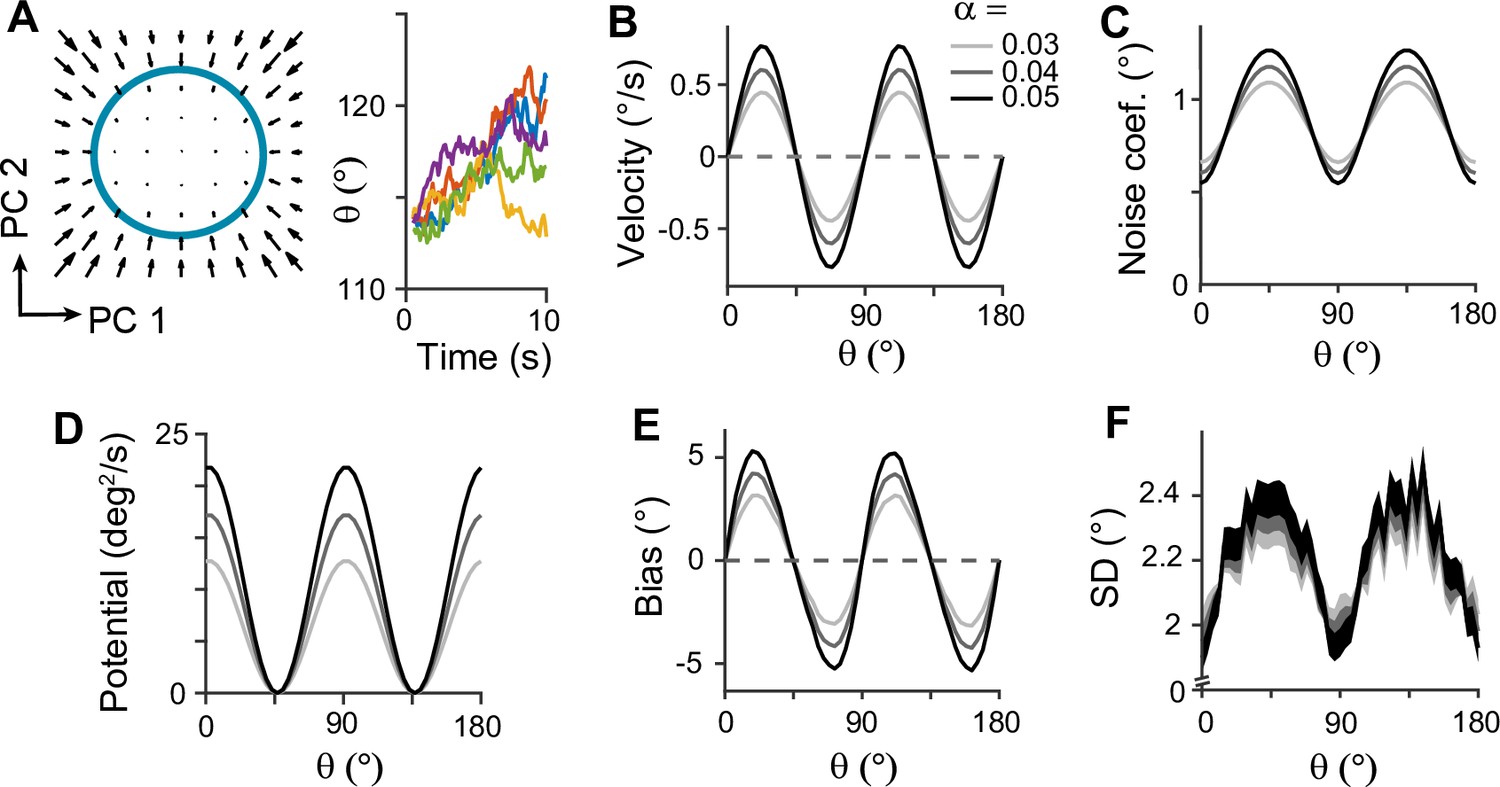
To further understand the mechanisms of generating the correct error patterns in sensory-memory interacting networks, we analyzed the network dynamics during the delay period. For this, we identified the low-dimensional manifold that has slow dynamics during the delay period, which corresponds to the memory states (Figure 5A). We projected the dynamics along this manifold to obtain the drift and diffusion terms (Figure 5A–C; Figure 5—figure supplement 1). The drift term shows similar patterns to cardinal repulsion (Figure 5B and E). Integrating this drift for orientation yields the energy function, which is minimum at the obliques (Figure 5D). This suggests that the network implements discrete attractor dynamics with attractors formed at the obliques. The diffusion term is also uneven – the noise amplitude is maximum at the obliques so that despite attraction toward them, the variance of errors can be maximum (Figure 5C and F). Note that while we use Poisson noise in all units to replicate neuronal spike variability, the pattern of noise coefficients remains unchanged even with constant Gaussian noise (Figure 5—figure supplement 2). This lower variance near cardinal orientations arises from more dispersed representations of stimuli, as the noise coefficient is inversely proportional to the distance between stimulus representations (Equation 21). Thus, the nonuniform characteristics of both drift and diffusion processes stem from the heterogeneous connections within the sensory module and align with the solution identified in low-dimensional memory models (Figure 1J–L).

Figure 5 with 2 supplements see all

Download asset Open asset

Low-dimensional dynamics along memory manifold and their dependence on heterogeneity degrees in the sensory module.

(A) Low-dimensional projection along the memory states. Left panel: The memory manifold projected to the first two principal components (PCs) associated with the vector fields. Right panel: Example drift-diffusion trajectories along the memory manifold starting at $θ = {112.5}^{\circ}$ . (**B, C**) Velocity (B) and noise coefficients (C) corresponding to drift and diffusion processes. Different gray scales represent different heterogeneity degrees in the sensory module, $α$ , in Figure 3B. The velocity with which the remembered orientation drifts to the obliques in a noise-free network (B). A larger noise coefficient around the obliques overcomes the underlying drift dynamics and causes the standard deviation pattern to reach its maxima at the obliques (C). (D) Equivalent one-dimensional energy potential derived from the velocity in (B). (**E, F**) Example bias (E) and standard deviation (F) patterns at 4 s into the delay. The shaded areas mark the ±s.e.m. of 1000 realizations.

Next, we examined how heterogeneity of connectivity in the sensory module affects the dynamics along the memory states. The magnitude of heterogeneity is denoted as α, and larger α represents a larger asymmetry of connectivity strengths at cardinal and oblique orientations (Figure 3B, left). When α increases, the asymmetry of drift and energy levels becomes more prominent, leading to a more rapid increase in bias (Figure 5B, D, and E). The diffusion term is also more asymmetric, compensating for stronger attraction to the obliques (Figure 5C). Thus, for larger α, the variability of errors is still higher at the obliques (Figure 5F). Another important parameter influencing error patterns is the intermodal connectivity strengths (Figure 6). Similar to the effect of increasing α, increases in feedforward or feedback strengths cause the energy levels to become more asymmetrical (Figure 6A and E), leading to a larger bias (Figure 6B and F). Conversely, the noise coefficient is less affected (Figure 6C and G), and the variance of errors decreases as the drift force becomes stronger (Figure 6D and H). Note that bias and variance patterns depend on the product of feedforward and feedback connections, denoted as γ, such that for a fixed γ, the error patterns remain similar (Figure 6I and J). In sum, the bias and variability of errors are determined by the degree of heterogeneity in the sensory module (α) and intermodal connectivity strengths (γ) as both α and γ affect the asymmetry of drift term similarly, while the asymmetry of diffusion term is more strongly influenced by α (Figure 6K and L).

Figure 6

Download asset Open asset

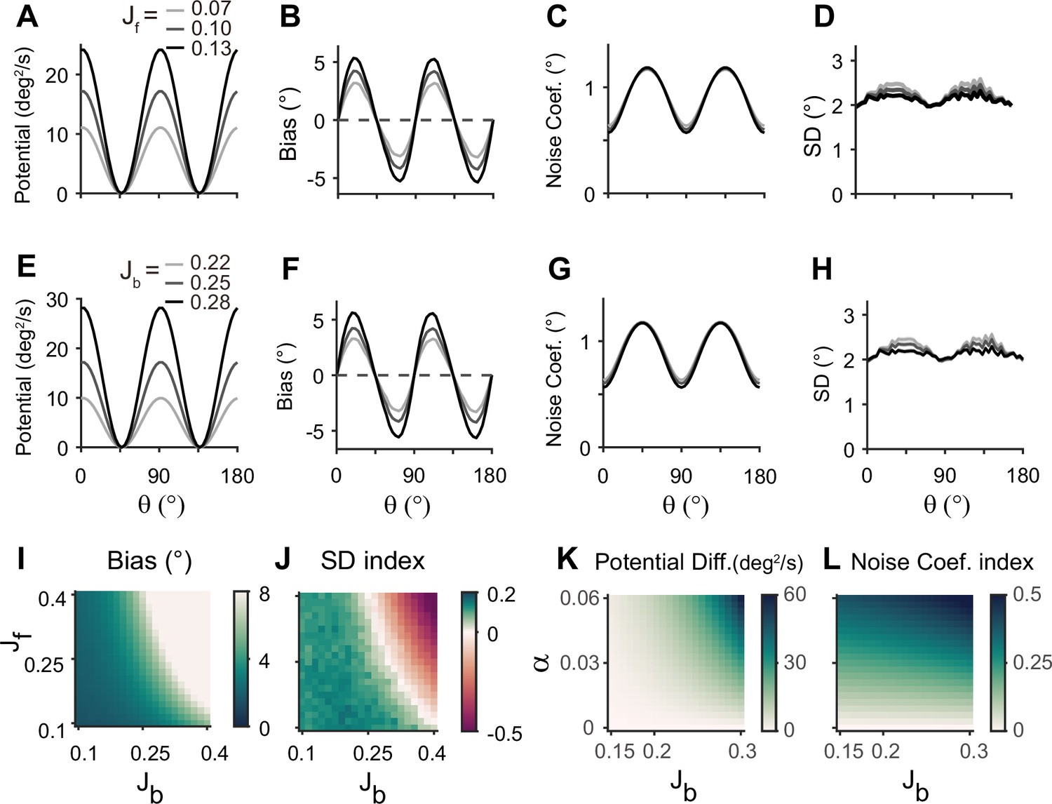
Error patterns and low-dimensional dynamics for different intermodal connectivity strengths.

(**A–J**) Low-dimensional dynamics and error patterns with varying feedforward and feedback connection strengths, denoted by J_f and J_b. (**K, L**) Potential differences and noise coefficient indices comparing low-dimensional dynamics at cardinal and oblique orientations for changing J_b and heterogeneity degree, $α$ . Increasing both feedforward (**A–D**) and feedback (**E–H**) connection strengths deepens the potential difference (**A, E, K**) and increases the bias (**B, F**), similar to the effects of $α$ increases in Figure 5D and E. In contrast, the profile of noise coefficients is less affected (**C, G, L**) and the SD pattern gets flattened with stronger drift (**D, H**). Bias and SD patterns depend on the product of feedforward and feedback connection strengths (**I, J**). Bias and SD are estimated at 4 s (**B, D, F, H**) or 1 s (**I,J**) into the delay and shaded areas mark the ±s.e.m. of 1000 realizations.

Importance of heterogeneously tuned inhibition

We showed that network models realizing sensory-memory interactions reproduce correct error patterns, where each module has a different connectivity structure. Previous work suggested that such a heterogeneous connection of the sensory system may arise from experience-dependent synaptic modification (Olshausen and Field, 1996; Zylberberg et al., 2011). For example, typical Hebbian learning is thought to potentiate connectivity strengths between neurons whose preferred stimuli are more frequently encountered. For orientations, cardinal directions are predominant in natural scenes. Thus, if experience-dependent learning occurs mainly at the excitatory synapses, the excitatory connections near cardinal orientations become stronger in the sensory module. This is opposite to the previously discussed case where the sensory module has the strongest connection at the obliques. With the strongest excitatory connections at cardinal orientations, the error patterns are reversed, resulting in cardinal attraction instead of repulsion, and the lowest variance occurs at the obliques.

Inhibitory synaptic connections can also be modified through learning (Vogels et al., 2013; Khan et al., 2018; Larisch et al., 2021). Here, we considered that experience-dependent learning exists in both excitatory and inhibitory pathways and similarly shapes their connectivity (Figure 7A). We assumed that excitatory and inhibitory connections are segregated and stronger near cardinal orientations (Figure 7B). We modulated the heterogeneity degree of both excitatory and inhibitory connections, denoted as α and β, respectively (Figure 7B–D). The ratio between α and β determines the direction and magnitude of bias and variance patterns (Figure 7C and D). For relatively larger α, the network shows cardinal attraction and minimum variance of errors at the obliques (Figure 7E). Reversely, for relatively larger β with stronger modulation in inhibitory connections, the network reproduced cardinal repulsion and minimum variance of errors at cardinal orientations, consistent with experiments (Figure 7F). With a larger difference between α and β, such patterns of bias and variance are potentiated and minimum Fisher information across orientations decreases, corresponding to memory loss (Figure 7C and D; Figure 7—figure supplement 1). Thus, this emphasizes the important role of heterogeneously tuned inhibition in shaping the sensory response for higher precision at cardinal orientations and enabling the sensory-memory interacting network to generate correct error patterns.

Figure 7 with 2 supplements see all

Download asset Open asset

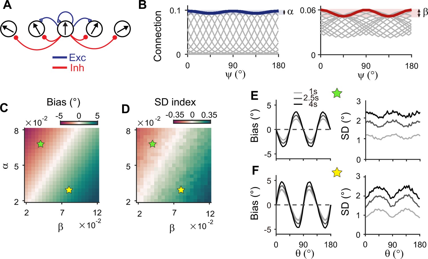
Stronger inhibitory synaptic modulation is required for correct error patterns.

(A) Segregation of excitatory (blue) and inhibitory (red) synaptic pathways. (B) Example excitatory (left) and inhibitory (right) connectivity strengths of the sensory module. The heterogeneity degrees of excitatory and inhibitory connections are denoted by $α$ and $β$ , respectively. Unlike combined excitation and inhibition in Figure 3B, the connectivity strengths are maximal around cardinal orientations. (**C, D**) Bias with stimulus at 22.5° (C) and standard deviation (SD) index (D) estimated at 1 s into the delay for different values of $α$ and $β$ . SD index compares the SD at the cardinal and oblique orientations (Methods). (**E, F**) Example bias (left) and SD (right) patterns when excitatory modulation overwhelms inhibitory modulation ( $α = 0.068, β = 0.04$ ; E) and when inhibitory modulation is stronger ( $α = 0.03, β = 0.08$ ; F). In (C) and (D), green (yellow) pentagrams mark the parameters used in (E) and (F). Stronger inhibitory modulation is required for correct bias and variance patterns (F) and green regions in (C and D). In (E) and (F), shaded areas mark the ±s.e.m. of 1000 realizations.

Comparison to alternative circuit structures

So far, we have shown the sufficiency of sensory-memory interacting networks with different connectivity structures featuring heterogeneous-homogeneous recurrent connections within each module. Here, we explore whether such architecture is necessary by comparing its performance with alternative circuit structures for sensory-memory interactions. One candidate mechanism involves having the heterogeneous sensory network maintain memory with a long intrinsic time constant, similar to having autapses (Seung et al., 2000). However, this model fails to replicate the evolution of error patterns during the delay period as a long intrinsic time constant slows down the overall dynamics, thus hindering the evolution of error patterns (Figure 7—figure supplement 2). Alternatively, we focused on a two-module network with variations in connectivity structure. We assumed that sensory and memory modules still serve their distinctive functions, namely, sensory encoding and memory maintenance, with weak/strong recurrent connections in sensory/memory modules. On the other hand, the heterogeneity of connections in other circuits might differ as homogeneous-homogeneous, homogeneous-heterogeneous, and heterogeneous-heterogeneous connections for sensory-memory modules.

Circuits with homogeneous connections in both sensory and memory modules are similar to previous continuous attractor models for working memory, such that the energy landscape and noise amplitude are uniform for all orientations (Figure 1D–F). Such architecture is not suitable as it generates no bias in errors and flat variance patterns. This leaves the latter two types of configurations, which require heterogeneous connections within the memory module. With a strong recurrent connection within the memory module, its heterogeneous activity pattern dominates overall activities in sensory-memory interacting networks, which makes it analogous to an isolated memory module. Thus, we examined the property of the memory module alone, which can maintain memory while generating heterogeneous responses without connection to the sensory module (Figure 8).

Figure 8

Download asset Open asset

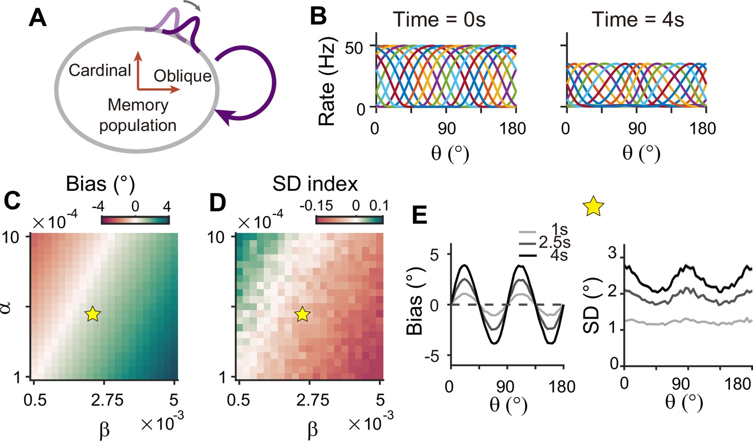
Network model with memory module only cannot reproduce correct error patterns.

(A) Schematics of one-module network with heterogeneous and strong recurrent connections that enable both efficient coding and memory maintenance. (B) Example tuning curves at the end of the stimulus epoch (left) and at 4 s into the delay epoch (right). (**C, D**) Bias with stimulus at 22.5° (C) and standard deviation (SD) index (D) estimated at 1 s into the delay for different heterogeneity degrees of excitatory and inhibitory connections, denoted by $α$ and $β$ . For the parameters that generate reasonable bias patterns, the SD index is always negative, which indicates that the SD pattern is inconsistent with experimental findings. (E) Bias (left), and SD (right) patterns in the delay. While the bias pattern is correct, the SD reaches maxima around cardinal orientations, unlike the experiments. In (C) and (D), the yellow pentagram marks the parameters used in (E).

To generate the correct bias pattern, we assumed that excitatory and inhibitory pathways in the memory module are stronger near cardinal orientations, as we previously considered for the sensory module in the sensory-memory interacting network (Figure 8A and B). However, memory circuits with heterogeneous connections have problems in maintaining the information and reproducing correct error patterns (Figure 8C–E). First, memory circuits alone require fine-tuning of heterogeneity whose range generating a moderate drift speed is at least one order of magnitude smaller than that of the two-module network (Figure 8C and D). Deviation from this range results in a fast drift toward oblique orientations, leading to rapid loss of information during the delay period (Figure 7—figure supplement 1). Second, despite the correct bias direction, the variance pattern is reversed such that the variance of errors is minimal at the oblique orientations (Figure 8E). Varying the heterogeneity in excitatory and inhibitory connections shows that such rapid drift and reversed error patterns are prevalent across different parameters (Figure 8C and D).

To understand why a heterogeneous memory circuit alone fails to reproduce correct error patterns, we compared its low-dimensional dynamics along the memory states to that of the sensory-memory interacting networks. For the network with a similar range of bias and variance on average, we compared their energy landscape and noise amplitude, which vary similarly in both networks with minimum energy level and maximum noise at the oblique orientations (Figure 9A–F). However, the energy difference between cardinal and oblique orientations in a single memory circuit model is bigger than that in a sensory-memory interacting network (Figure 9C, left in Figure 9G, H). In contrast, the difference in noise amplitude is smaller (Figure 9D–F, right in Figure 9G, H). The attraction at the obliques is much stronger, leading to the correct bias patterns, but too rapid an increase. Also, smaller differences in noise amplitude cannot overcome strong drift dynamics, leading to the minimum variance of errors at the obliques and reversed variance patterns. Even for different types or levels of noise, such as Gaussian noise with varying amplitude, distinctive error patterns in one-module and two-module networks are maintained (Figure 9—figure supplement 1).

Figure 9 with 1 supplement see all

Download asset Open asset

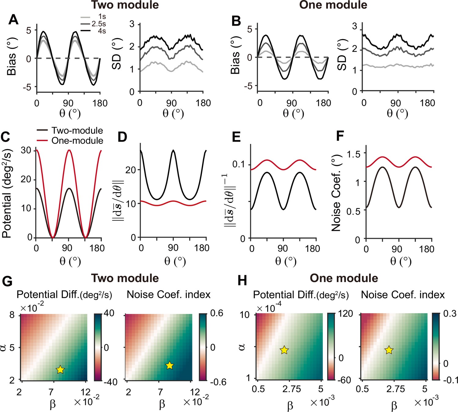
Comparison of low-dimensional dynamics between two-module and one-module network models.

(**A, B**) Bias and standard deviation (SD) patterns of two-module (A) and one-module (B) networks, adapted from Figure 7F and Figure 8E, respectively. The averages of bias and SD over different $θ$ at 4 s into the delay are similar in the two networks. (**C–F**) Low-dimensional dynamics of two-module (black) and one-module (red) networks. In both networks, the energy potential (C), the distance between stimulus representation, $∥ {\bar{s}}^{'} (θ) ∥$ and its inverse determining noise coefficients (**D, E**; Equation 21), and the noise coefficients (F) exhibit similar profiles. However, the two-module network has a shallower potential (C) but larger heterogeneity in $∥ {\bar{s}}^{'} (θ) ∥$ and the noise coefficient profile (**D–F**). These differences make it possible for the SD to become smaller around cardinal orientations in the two-module network (right in A), while drift dynamics overwhelm and the SD pattern is opposite to that of the noise coefficient in the one-module network (right in B). (**G, H**) Potential difference (left) and index of noise coefficients (right) comparing low-dimensional dynamics at the cardinal and oblique orientations in two-module (G) and one-module (H) networks. The two-module network shows a smaller potential difference and more heterogeneous noise coefficients over a broad range of heterogeneity (see the color bars in G and H).

For an intuitive understanding of how connectivity heterogeneity affects the degrees of asymmetry in drift and diffusion differently in one-module and two-module networks, consider a simple case where only the excitatory connection exhibits heterogeneity, the degree of which is denoted by α. For memory maintenance, the overall recurrent connections need to be strong enough to overcome intrinsic decay, simplified to w=1. In the one-module network, α in the memory module causes deviations from perfect tuning, creating potential differences at cardinal and oblique orientations as 1±α. In the two-module network, with w=1 fulfilled by the memory module, α in the sensory module acts as a perturbation. The effect of α is modulated by the intermodal connectivity strengths, denoted by γ, and potential differences at cardinal and oblique orientations can be represented as 1±γα. Thus, while a relatively large α leads to too fast drift in the one-module network, the drift speed in the two-module network could remain modest with small γ<1. Conversely, even with small γ, the asymmetry of noise coefficients can be large enough to produce correct variance patterns because the noise coefficient is more strongly influenced by α in the two-module network (Figure 6). In sum, compared to a heterogeneous memory circuit alone, interactions between heterogeneous sensory and homogeneous memory modules are advantageous due to an additional degree of freedom, intermodal connectivity strengths, which allows better control of energy and noise difference at cardinal and oblique orientations.

Discussion

While higher association areas have long been considered as a locus of working memory (Roussy et al., 2021; Mejías and Wang, 2022), recent human studies found memory signals in early sensory areas, prompting a re-evaluation of their role in working memory (Xu, 2020; Adam et al., 2022). Our work extends the traditional memory models (Wang, 2001; Khona and Fiete, 2022) with novel insights into the significance of stimulus-specific sensory areas. We showed how sensory-memory interactions can elucidate changes in the internal representation of orientation stimuli and their behavioral readout during memory tasks. The observed error patterns suggest that the network meets two demands simultaneously: efficient encoding that reflects natural statistics and memory maintenance for successful retrieval of stimuli after a delay. Achieving both demands for orientation stimuli conflicts in a one-module network. Efficient encoding necessitates asymmetrical connections, resulting in inconsistent bias and variance patterns and overly rapid drift in the one-module network unless fine-tuned. In contrast, connecting sensory and memory modules can generate error patterns correctly and with less need for fine-tuning heterogeneity for slow drift. Efficient coding of natural statistics in the sensory module underscores the role of inhibitory plasticity. Low-dimensional projection onto memory states reveals that drift and diffusion processes governing working memory dynamics closely resemble the bias and variance patterns derived under Bayesian sensory models. It also elucidates how the magnitudes of bias and variance change depending on the heterogeneity of sensory connections and intermodal connectivity strengths.

Our model makes testable predictions to differentiate two-module and one-module networks using perturbation, such as transcranial magnetic stimulation (TMS). Many studies have found that during the delay period, TMS can intervene with the feedforward signal from sensory areas through which working memory is consolidated (van de Ven et al., 2012) (but see Adam et al., 2022, for mixed effects of TMS and related debate). Under such perturbations, the ability to maintain information in the memory module will not be affected due to strong recurrent connections in both two-module and one-module networks. However, we expect different effects on bias patterns — in the two-module network, the bias will stop systematically drifting toward the obliques, reducing systematic repulsion (Figure 10). This accompanies the nonincreasing heterogeneity of tuning curves after the disruption, marked by their tuning width indices (see Methods). In contrast, in the one-module network, perturbation does not incur changes in error patterns as memory activities are less dependent on the sensory module during the delay period. Thus, perturbation studies can be used to reveal the role of the sensory module in shaping the error patterns during working memory. Note that our model cannot predict the effects of distractors during working memory, as such effects do not experimentally lead to changes in error patterns (Rademaker et al., 2019). The effect of distractors and direct intervention in the intermodule connections may differ due to potential differences in the encoding of distractors compared to task-relevant stimuli. More advanced models are required to comprehensively understand the influence of distractors and the processing of ongoing visual stimuli or the storage of multiple stimuli.

Figure 10

Download asset Open asset

Effect of perturbations in sensory-memory interaction on error patterns.

(**A, B**) Example bias (A) and standard deviation (B) patterns when we assumed that transcranial magnetic stimulation (TMS) is applied to interrupt the feedforward signal from 2.5 s into the delay. Shaded areas mark the ±s.e.m. of 1000 realizations. (**C, D**) Evolution of bias with example cue orientation at $θ = 18^{\circ}$ (C) and the tuning width indices in the memory network (WI; C) representing the asymmetry of tuning widths at cardinal and oblique orientations (Methods). Two vertical dashed lines mark the end of the stimulus epoch and the beginning of TMS disruption, respectively. Solid and dashed curves correspond to with and without perturbations, respectively. Both bias (C) and WI (D) stop increasing when TMS is on (**C, D**).

Our work suggests biologically plausible network mechanisms for the previously postulated efficient coding and Bayesian inference principles, relating network connectivity to tuning properties and error patterns. Previous normative explanations for systematic bias observed in perception tasks also suggested possible neural substrates for efficient coding, such as asymmetrical gain, width, or density of tuning curves across stimulus features (Ganguli and Simoncelli, 2014; Wei and Stocker, 2015). Our work narrowed the mechanism to denser and narrower tuning curves at cardinal orientations, consistent with neurophysiological recordings in the visual cortex (Li et al., 2003; Kreile et al., 2011; Shen et al., 2014). We implemented a population vector decoder reflecting neuronal preferred orientations, which approximates Bayesian optimal readout (Fischer, 2010). Compared to a previous work adapting efficient coding theories with static tuning curves to account for error patterns in working memory tasks (Taylor and Bays, 2018), our extension to memory processes demonstrated how neural activities and behavior readout change dynamically during the delay period. Notably, recent work combined dynamic change of signal amplitude with static tuning curves to capture different time courses of estimation precision during sensory encoding and memory maintenance (Tomić and Bays, 2023). Our network models embody such phenomenological models as the networks exhibit changes in overall firing rates after the stimulus offset.

Like our study, a few recent studies have employed attractor dynamics to explain dynamic error patterns observed for visual color memory (Panichello et al., 2019; Pollock and Jazayeri, 2020; Eissa and Kilpatrick, 2023). Behavior studies showed attractive bias and minimum variance around the prevalent colors, which one-module discrete attractor models could reproduce. However, these models cannot be generalized to other visual stimuli, such as orientations, spatial locations, or directions, of which the responses show repulsive bias away from the common stimuli (Wei and Stocker, 2017). Also, a one-module network storing color memory requires fine-tuned heterogeneity for moderate drift speed. While the desired low-dimensional manifold and drift dynamics can be engineered in the one-module network (Pollock and Jazayeri, 2020), its biological mechanism needs further investigation. The two-module network considered in our study also requires fine-tuning of homogeneity in the memory module and heterogeneity in the sensory module. However, the condition of asymmetrical connections in the sensory module is less stringent as they have a weaker influence on the entire dynamics than those in the memory module. Fine-tuning of homogeneous connections in the memory module can be mediated through activity-dependent plasticity, such as short-term facilitation (Itskov et al., 2011; Hansel and Mato, 2013; Seeholzer et al., 2019) or long-term plasticity (Renart et al., 2003; Gu and Lim, 2022). Also, recent work showed that continuous attractors formed under unstructured, heterogeneous connections are robust against synaptic perturbations (Darshan and Rivkind, 2022). Thus, the two-module networks can control the drift speed better with possible additional mechanisms that promote homogeneous memory states. It needs further exploration whether they can be generalized to other stimuli like color, possibly involving additional categorical structures (Hardman et al., 2017; Pratte et al., 2017).

Our current study is limited to the dynamic evolution of memory representation for a single orientation stimulus and its associated error patterns, which does not capture nuanced error patterns in broader experimental settings (Hahn and Wei, 2024). For instance, while shorter stimulus presentations with no explicit delay led to larger biases experimentally, our current model, which starts activities from a flat baseline, shows an increase in bias throughout the stimulus presentation (de Gardelle et al., 2010). Additionally, the error variance during stimulus presentation is almost negligible compared to that during the delay period, as the external input overwhelms the internal noise. These mismatches during stimulus presentation have minimal impact on activities during the delay period when the internal dynamics dominate. Nonetheless, the model needs further refinement to accurately reproduce activities during stimulus presentation, possibly by incorporating more biologically plausible baseline activities. Also, a recent Bayesian perception model suggested different types of noise like external noise or variations in loss functions that adjust tolerance to small errors may help explain various error patterns observed across different modalities (Hahn and Wei, 2024). Even for memories involving multiple items, noise can be critical in determining error patterns, as encoding more items might cause higher noise for each individual item (Chunharas et al., 2022).

The modularity structure in the brain is thought to be advantageous for fast adaptation to changing environments (Simon, 1995; Cole et al., 2013; Frankland and Greene, 2020). Recent works showed that recurrent neural networks trained for multiple cognitive tasks form clustered neural activities and modular dynamic motifs to repurpose shared functions for flexible computation (Yang et al., 2019; Driscoll et al., 2022). Resonant with these computational findings, an fMRI study showed that shared representation across distinct visual stimuli emerges during the delay period (Kwak and Curtis, 2022). Although our work focuses on a single task, it highlights the necessity of having dedicated sensory and memory modules, and a memory module with ring geometry can be repurposed for various visual stimuli such as motion, spatial location, and color. It is reminiscent of the flexible working memory model, which proposes connections between multiple sensory modules and a control module (Bouchacourt and Buschman, 2019). However, a key distinction lies in the role of the control module. Unlike the flexible working memory model that loses memory without sensory-control interactions, our work suggests that the memory module can independently maintain memory, while interaction with the sensory module continuously shapes the internal representation, potentially consolidating prior beliefs regarding natural statistics. The sensory-memory interaction and network architecture derived from dynamic changes of single stimulus representation can be a cornerstone for future studies in more complex conditions, such as under the stream of visual inputs (Xu, 2020; Adam et al., 2022) or with high or noisy memory loads (Bays et al., 2022).

Methods

Low-dimensional attractor models

To illustrate error patterns in different low-dimensional attractor models shown in Figure 1, we considered a one-dimensional stochastic differential equation given as

d θ_{t} = μ (θ_{t}) d t + σ (θ_{t}) d W_{t},

where $θ_{t}$ and $W_{t}$ are orientation and standard Brownian motion at time t, respectively. We assumed that the drift and noise coefficients μ and σ only depend on $θ_{t}$ , where $σ = \sqrt{2 D}$ with diffusion coefficient $D$ .

For continuous attractor models in Figure 1D–F, μ and σ were set to be constant as $μ = 0$ and $σ = 2 °$ . For discrete attractor models in Figure 1G–L, we assumed that the energy function $U (θ_{t})$ is proportional to $c o s (4 θ_{t})$ (Figure 1G and J) so that the drift term $μ (θ_{t}) = \sin (4 θ_{t})$ with $μ (θ_{t}) = - \frac{d U}{d θ_{t}}$ . In these attractor models, the constant noise in Figure 1G–I is $σ = 2 °$ and the nonuniform noise in Figure 1J–L is $σ = 2 ° (1 - c o s (4 θ_{t}))$ . The biases and standard deviation (SD) of errors were plotted at T=1, 2, and 3 with 50,000 iterations. For the numerical simulation, dt =0.01.

Bayesian sensory models and extension

In Figure 2, we first constructed the sensory inference process, which receives orientation input $θ$ , forms a corresponding noisy sensory representation $m$ given $θ$ , and then infers $\hat{θ}$ as an estimate of the input orientation from the encoded representation $m$ . This inference is made in a Bayesian manner based on likelihood function $p (m | θ)$ and orientation prior $q (θ)$ .

To construct $p (m | θ),$ we followed the procedure given in Wei and Stocker, 2015, and the summary is as follows. We started from the sensory space of $\tilde{θ}$ where both discriminability and Fisher information $J (\tilde{θ})$ are uniform, and all likelihood functions $p (m | \tilde{θ})$ are homogeneous von Mises functions. And since $J (θ) \propto (q (θ))^{2}$ under the efficient coding condition, the sensory space of $\tilde{θ}$ and the stimulus space of $θ$ can be mapped by forward and backward mappings $F (θ)$ and $F^{- 1} (\tilde{θ})$ , where $F (θ)$ is the cumulative distribution function of prior $q (θ)$ . Thus, likelihood functions $p (m | θ)$ can be obtained by taking homogeneous von Mises likelihoods in the sensory space and transforming them back to the stimulus space using $F^{- 1}$ . To sum up the upper half of the procedural diagram in Figure 2A, the sensory module receives $θ$ , encodes it in $m$ following $p (m | θ)$ , and decodes $\hat{θ}$ using likelihood functions and prior $q (θ)$ .

As an extension to include a memory process, the decoded $\hat{θ}$ is passed on to the memory module, where $\hat{θ}$ is maintained with the addition of memory noise $ξ$ . The output of the memory module, $\hat{θ} + ξ$ , is fed back to the sensory module as the new input. This completes one iteration of sensory-memory interaction. The whole process is then repeated recursively, resulting in increased biases and standard deviations in the $θ$ statistics at subsequent iterations (call them $θ_{i}$ for the input of iteration $i$ ).

For Figure 2B and C, we set the von Mises sensory-space likelihoods to be $p (m | \tilde{θ}) \propto e x p (κ_{m} c o s (m - \tilde{θ}))$ , with $κ_{m} = 250$ . These likelihood functions are transformed by $F^{- 1} (\tilde{θ}) = {\int q (θ)}^{- 1}$ , where $q (θ) = 3 + c o s (4 θ)$ . Each internal representation $m$ is sampled from $p (m | θ)$ , after which $\hat{θ}$ is estimated as the mean of the posterior $p (θ | m) q (θ)$ . With the parameters chosen above, the inferred samples of $\hat{θ}$ after the first sensory iteration have a circular standard deviation of $σ_{θ} \approx 1.3 °$ at cardinal orientations. To have comparable memory and sensory noise levels, we set the memory noise as $ξ ~ N (0, {(1.3 °)}^{2})$ which is added on top of the sensory outputs. Thus, the memory outputs of the first iteration $θ_{1} = {\hat{θ}}_{1} + ξ$ have a standard deviation of 1.84^o at the cardinals. The first three iterations’ memory output statistics are plotted in Figure 2C, i.e., bias( $θ_{1}$ ), bias( $θ_{2}$ ), bias( $θ_{3}$ ), and SD( $θ_{1}$ ), SD( $θ_{2}$ ), SD( $θ_{3}$ ). The statistics were computed from 10,000 iterations of the simulation. The magnitude of biases and standard deviations vary for different sensory or memory noise levels, while the overall patterns and the increasing temporal trend are unchanged (not shown).

Firing rate models

For network models, we considered sensory circuits with heterogeneous connections (Figure 3), memory circuits with homogeneous connections (Figure 3) and heterogeneous connections (Figures 8 and 9), and sensory-memory interacting circuits (Figures 4—7, 9, and 10). In all cases, the activities of neurons are described by their firing rates and synaptic states, denoted by $r$ and $s$ . For columnar structure encoding orientation stimuli, we indexed the neurons by uniformly assigning them indices $ψ_{i} = \frac{(i - 1)}{N} \times 180^{\circ}$ for $i$ from 1 to $N$ , where $N$ is the number of neurons in each population. For sensory or memory networks alone, the dynamics of neuron $i$ are described by the following equations:

\begin{array}{ll} r_{k}^{i} & = f_{k} (\sum_{j} W_{k}^{i j} s_{k}^{j} + I_{ext, k}^{i}) \\ τ {\dot{s}}_{k}^{i} & = - s_{k}^{i} + r_{k}^{i} + ξ_{k}^{i} \end{array}

where the superscripts $i$ and $j$ are the neuronal indices, and the subscript $k$ is either $s$ or $m$ , representing sensory or memory circuits. For the sensory-memory interacting network, the dynamics are given as

\begin{array}{ll} r_{s} & = f_{s} (W_{s} s_{s} + W_{b} s_{b} + I_{ext,s}) \\ r_{m} & = f_{m} (W_{m} s_{m} + W_{f} s_{f} + I_{ext,m}) \\ τ {\dot{s}}_{k} & = - s_{k} + r_{s} + ξ_{k}, for k = s or f \\ τ {\dot{s}}_{l} & = - s_{l} + r_{m} + ξ_{l}, for l = m or b \end{array},

where activities and synaptic inputs are represented in the vector and matrix multiplication form, shown in bold cases. The additional subscripts $f$ and $b$ represent feedforward and backward connections between sensory and memory modules.

In both Equations 2 and 3, $s (t)$ is the low pass filtered $r (t)$ with synaptic time constant $τ$ and with the addition of $ξ$ approximating Poisson noise. We modeled $ξ$ as the Gaussian process with covariance $⟨ξ^{i} (t) ξ^{j} (t `)⟩ = r^{i} (t) δ_{i j} δ (t - t `)$ , following Burak and Fiete, 2012. We assumed that the rate dynamics are relatively fast such that $r (t)$ equals the input current-output rate transfer function f. The input current is the sum of external input $I_{e x t}$ and the synaptic currents from other neurons in the network, which are the postsynaptic states $s^{j}$ weighted by synaptic strengths $W^{i j}$ . The transfer function f has the Naka-Rushton form (Wilson, 1999) given as

f (x) = f_{m a x} \frac{{(x - T)}^{q}}{w^{q} + {(x - T)}^{q}} \cdot {[x - T]}_{+},

where ${[\cdot]}_{+}$ denotes the linear rectification function. The transfer functions differ in the sensory and memory modules, denoted as $f_{s}$ and $f_{m}$ , respectively.

Synaptic inputs in network models

Note that for all network models, we only considered excitatory neurons under the assumption that the inhibitory synaptic pathways have relatively fast dynamics. Thus, recurrent connectivity strengths, $W_{s}$ and $W_{m}$ , within sensory and memory modules, reflect summed excitation and inhibition, and thus, can have either positive or negative signs. On the other hand, we assumed that intermodal interactions, $W_{f}$ and $W_{b}$ , are dominantly excitatory and, thus, can be only positive.

All $W$ ’s can be defined using neuronal indices of post- and presynaptic neurons as

W^{i j} = \frac{1}{N} J (ψ_{i}, ψ_{j}) .

For $W_{s}$ without segregating excitation and inhibition in Figures 3—6, $N$ is the population size of sensory module, $N_{s}$ , and $J_{s}$ is the sum of a constant global inhibition and a short-range excitatory connection as

J_{s} (ψ_{i}, ψ_{j}) = - J_{I, s} + J_{E,s} (1 - α c o s 4 ψ_{i}) e^{- \frac{{(ψ_{i} - ψ_{j})}^{2}}{λ_{E,s}^{2}}},

where $α > 0$ represents the heterogeneity degree of excitatory connectivity, and $λ_{E}$ is the width of local excitatory connections.

When we segregated excitation and inhibition and considered the heterogeneity of inhibitory connection in Figures 7—10, Equation 6 is replaced with

J_{s} (ψ_{i}, ψ_{j}) = - J_{I, s} (1 + β c o s 4 ψ_{i}) e^{- \frac{{(ψ_{i} - ψ_{j})}^{2}}{λ_{I,s}^{2}}} + J_{E, s} (1 + α c o s 4 ψ_{i}) e^{- \frac{{(ψ_{i} - ψ_{j})}^{2}}{λ_{E,s}^{2}}},

where $β > 0$ is the degree of heterogeneity of inhibitory connections. Note the signs of modulation change in Equations 6 and 7 such that when only excitation is modulated in Equation 6, the connectivity strengths near the obliques are strong. In contrast, when excitation and inhibition are both modulated in Equation 7, the connectivity strengths near cardinal orientations are strong.

For the memory module, $N$ is the population size of the memory module, $N_{m}$ in Equation 5. Without heterogeneity in Figures 3—7 and 10, $J_{m}$ is defined as

J_{m} (ψ_{i}, ψ_{j}) = - J_{I, m} e^{- \frac{{(ψ_{i} - ψ_{j})}^{2}}{λ_{I,m}^{2}}} + J_{E, m} e^{- \frac{{(ψ_{i} - ψ_{j})}^{2}}{λ_{E,m}^{2}}} .

In contrast, for the one-module network model in Figure 8, the connectivity of the memory module is heterogeneous, as in the sensory module in Equation 1, and is defined as

J_{m} (ψ_{i}, ψ_{j}) = - J_{I, m} (1 + β \cos 4 ψ_{i}) e^{- \frac{{(ψ_{i} - ψ_{j})}^{2}}{λ_{I,m}^{2}}} + J_{E, m} (1 + α \cos 4 ψ_{i}) e^{- \frac{{(ψ_{i} - ψ_{j})}^{2}}{λ_{E,m}^{2}}} .

The feedforward and feedback connectivity are similarly defined as

\begin{array}{cc} W_{f}^{i j} & = \frac{1}{N_{s}} J_{f} e^{- {(ψ_{m i} - ψ_{s j})}^{2} / λ_{f}^{2}} \\ W_{b}^{i j} & = \frac{1}{N_{m}} J_{b} e^{- {(ψ_{s i} - ψ_{m j})}^{2} / λ_{b}^{2}} . \end{array}

Note the connectivity strength is normalized by the size of the presynaptic population so that the total synaptic current remains the same for different population sizes.

For the external inputs with orientation $θ$ , $I_{ext,s}$ in the sensory module is modeled as

I_{ext,s}^{i} (θ) = C (1 - 2 ε + 2 ε e^{- {(ψ_{i} - θ)}^{2} / λ_{ext,s}^{2}}),

where $ε \in (0, 0.5]$ determines the stimulus tuning of the input, $λ_{ext,s}$ determines the width, and $C$ describes the contrast (Hansel and Sompolinsky, 1998).

For the memory network not connected to the sensory module in Figures 3 and 8, we assumed stimulus-specific input as

I_{ext, m}^{i} (θ) = \frac{1}{2} (\cos (2 (ψ_{i} - θ)) + 1) + I_{c, m},

where $I_{c, m}$ is a constant background input. When the memory module receives the inputs from the sensory population in Figures 4—7 and 10, we assumed $I_{ext, m}^{i} (θ)$ is constant as $I_{c, m}$ .

Analysis of network activities

We used population vector decoding to extract the internal representation of orientation and quantified how such representation deviated from the original stimulus. We also examined how tuning properties and Fisher information change during the delay period.

Note that while we indexed neurons uniformly with $ψ_{i}$ between 0° and 180°, the maximum of the tuning curve of neuron $ψ_{i}$ can change dynamically and differ from $ψ_{i}$ . We defined the preferred feature (PF) of neuron $i$ as the maximum of its tuning curve when the tuning curve reaches a steady state in the presence of external input. For numerical estimation, we set the stimulus-present encoding epoch to 5 s to obtain the steady states of tuning curves. The tuning width is given as the full width at half maximum (FWHM) of the tuning curve. To estimate PF and FWHM, we did a cubic spline interpolation to increase the number of sample orientations to 1000. The tuning width index (WI) is given as

W I = \frac{F W H M (ψ = 45^{\circ}) - F W H M (ψ = 0^{\circ})}{F W H M (ψ = 45^{\circ}) + F W H M (ψ = 0^{\circ})} .

To estimate the internal representation of orientation in the network models, denoted as $\hat{θ}$ , we utilized the population vector decoder (Georgopoulos et al., 1986)

\hat{θ} (t) = \frac{1}{2} A r g (\sum_{j = 1}^{N} e x p {2 i r^{j} (t) {\tilde{θ}}_{j}} / \sum_{j = 1}^{N} r^{j}),

where $N$ denotes the number of neurons and ${\tilde{θ}}_{j}$ denotes the PF of neuron $j$ . The orientation is always decoded from the memory network tuning curves $r_{m} (t)$ except for Figure 10A. The estimation bias $b (θ, t) = E [\hat{θ} (t)] - θ$ . Since the bias is typically small enough, we computed the estimation standard deviation (SD) as the SD of bias using linear statistics. The SD index is defined as

S D i n d e x = \frac{S D (θ = 45^{\circ}) - S D (θ = 0^{\circ})}{S D (θ = 45^{\circ}) + S D (θ = 0^{\circ})} .

The Fisher information (FI) is estimated by assuming that the probability density function $p (r ∣ θ)$ is Gaussian as

p (r_{m}^{i} | θ) = \frac{1}{\sqrt{2 π} σ_{i} (θ)} e^{\frac{{(r_{m}^{i} (θ) - E [r_{m}^{i} (θ)])}^{2}}{2 σ_{i}^{2} (θ)}},

where $σ_{i}^{2} (θ) = V a r (r_{m}^{i} (θ))$ denotes the variance of the firing rate of memory neuron $i .$ Thus, we can estimate the FI of memory neuron $i$ based on the empirical mean and variance of the firing rate at time $t$ as

F I (ψ_{i}, t) = \frac{{(\partial E [r_{m}^{i} (θ, t)] / \partial θ)}^{2}}{σ_{i}^{2} (θ, t)},

and the total FI is the summation of the FI of all memory neurons, given as $F I (t) = \sum_{i} F I (ψ_{i}, t)$ .

Drift and diffusivity in network models

Although the modulation breaks the continuity of the ring attractor and forms two discrete attractors at the obliques, there is still a one-dimensional trajectory $\bar{s} (θ)$ to which the noise-free dynamics quickly converge. We can linearize the system in the vicinity of this trajectory if the noise is small (Burak and Fiete, 2012). Note that the dynamics of the synaptic variables in Equation 3 can be put into the following form:

τ \dot{s} = - s + ϕ (W s + h) + ξ,

and by linearizing around the stable trajectory $s = \bar{s}$ , we get

τ \dot{δ s} = K δ s + ξ,

where we have ignored the zeroth- and higher-order terms. The drift velocity $μ (θ)$ is estimated by projecting the noise-free dynamics along the normalized right eigenvector u of K with the largest real part of the eigenvalue

μ (θ) = \frac{1}{τ ∥ \bar{s}' (θ) ∥} u^{T} (θ) [- \bar{s} (θ) + ϕ (W \bar{s} (θ) + h (θ))] .

The coefficient of diffusion can be obtained in the same way

2 D (θ) = \frac{1}{{(τ ∥ {\bar{s}}^{'} (θ) ∥)}^{2}} \sum_{i} u_{i}^{2} (θ) ϕ_{i} (\sum_{j} W_{i j} {\bar{s}}_{j} (θ) + h_{i}) .

The noise coefficient is given as $σ = \sqrt{2 D}$ . Hence, we have reduced the high-dimensional dynamics to a simple one-dimensional stochastic differential equation as in Equation 1 as

d θ = μ (θ) d t + σ (θ) d W_{t},

and the potential $U (θ)$ is obtained by the relation $\frac{d U}{d θ} = - μ (θ)$ . To quantitatively measure the heterogeneity of noise coefficient across different orientations, we define the noise coefficient index as follows:

N o i s e C o e f . i n d e x = \frac{σ (θ = 45^{\circ}) - σ (θ = 0^{\circ})}{σ (θ = 45^{\circ}) + σ (θ = 0^{\circ})} .

Network parameters and simulations

Unless otherwise specified, $N_{s} = N_{m} = 300$ , $τ = 10 m s$ . The connectivity parameters are $J_{E, s} = 0.6, J_{I,s} = 0.35, J_{E,m} = 1, J_{I,m} = 0.17, J_{f} = 0.1, J_{b} = 0.25, λ_{E,s} = 0.36 π, λ_{I,s} = 1.1 π, λ_{E, m} = 0.2 π,$ $λ_{I, m} = 0.6 π, λ_{f} = λ_{b} = 0.17 π$ . For the external input, we set $C = 4, ε = 0.2$ , and $λ_{ext,s} = 0.3 π$ . For the modulation of the sensory network, unless otherwise specified, we set $α = 0.04$ when only the excitatory plasticity is considered, and $α = 0.03, β = 0.08$ when the inhibitory plasticity is added. As for the modulation of the single-layer memory network, we set $α = 5 \times 10^{- 4}, β = 2.4 \times 10^{- 3}$ . For the transfer function, $f_{max} = 100, T = 0.1, q = 2, w = 6$ for sensory $f_{s}$ , and $f_{max} = 100, T = 0.1, q = 1.5, w = 6.6$ for memory $f_{m}$ .

We uniformly sampled 50 cue orientations in $[0^{\circ}, 180^{\circ}]$ . The visual cue lasts for 0.5 s except for the estimation of the PFs. In the grid parameter search figures, the delay epochs last for 1 s. In Figure 3, we set $α = 0.07$ . In Figure 5A, the manifold corresponds to the synaptic variables at 4 s into the delay with $α = 0.05$ . We uniformly sampled 100 cue orientations for the manifold.

To compute the drift velocity and noise coefficient in Figures 5, 6, and 9, we use the stable trajectory $\bar{s} (θ)$ at 1 s into the delay to ensure the fast transient dynamics induced by stimulus offset fully decays. The stable trajectory is parameterized by the 50 cue orientations to numerically compute ${\bar{s}}^{'} (θ) .$

All simulations of ordinary or stochastic differential equations of the network models were done using the Euler method with $d t = 1 m s$ . We checked that similar results hold for smaller $d t$ . Example bias and standard deviation patterns were estimated from 1000 independent realizations. The Fisher information patterns were estimated from 3000 independent realizations. The grid search of maximum bias at $θ = {22.5}^{\circ}$ and standard deviation index were computed from 3000 realizations.

All simulations were run in MATLAB. The code is available at GitHub (copy archived at Yang, 2024).

Data availability

The current manuscript is a computational study, so no data have been generated for this manuscript. The code is available at GitHub (copy archived at Yang, 2024).

References

Book
(2022) Evidence for, and challenges to, sensory recruitment models of visual working memory
In: Brady TF, Bainbridge WA, editors. Visual Memory. Routledge. pp. 5–25.

https://doi.org/10.4324/9781003158134-2
- Google Scholar
1. Bae GY
(2021) Neural evidence for categorical biases in location and orientation representations in a working memory task
NeuroImage 240:118366.

https://doi.org/10.1016/j.neuroimage.2021.118366
- PubMed
- Google Scholar
1. Bays PM
(2014) Noise in neural populations accounts for errors in working memory
The Journal of Neuroscience 34:3632–3645.

https://doi.org/10.1523/JNEUROSCI.3204-13.2014
- PubMed
- Google Scholar
Preprint
1. Bays P
2. Schneegans S
3. Ma WJ
4. Brady TF
(2022) Representation and Computation in Working Memory
PsyArXiv.

https://doi.org/10.31234/osf.io/kubr9
- Google Scholar
1. Bouchacourt F
2. Buschman TJ
(2019) A flexible model of working memory
Neuron 103:147–160.

https://doi.org/10.1016/j.neuron.2019.04.020
- PubMed
- Google Scholar
1. Burak Y
2. Fiete IR
(2009) Accurate path integration in continuous attractor network models of grid cells
PLOS Computational Biology 5:e1000291.

https://doi.org/10.1371/journal.pcbi.1000291
- PubMed
- Google Scholar
1. Burak Y
2. Fiete IR
(2012) Fundamental limits on persistent activity in networks of noisy neurons
PNAS 109:17645–17650.

https://doi.org/10.1073/pnas.1117386109
- PubMed
- Google Scholar
(2022) An adaptive perspective on visual working memory distortions
Journal of Experimental Psychology. General 151:2300–2323.

https://doi.org/10.1037/xge0001191
- PubMed
- Google Scholar
1. Cole MW
2. Reynolds JR
3. Power JD
4. Repovs G
5. Anticevic A
6. Braver TS
(2013) Multi-task connectivity reveals flexible hubs for adaptive task control
Nature Neuroscience 16:1348–1355.

https://doi.org/10.1038/nn.3470
- PubMed
- Google Scholar
(2000) Synaptic mechanisms and network dynamics underlying spatial working memory in a cortical network model
Cerebral Cortex 10:910–923.

https://doi.org/10.1093/cercor/10.9.910
- PubMed
- Google Scholar
1. Darshan R
2. Rivkind A
(2022) Learning to represent continuous variables in heterogeneous neural networks
Cell Reports 39:110612.

https://doi.org/10.1016/j.celrep.2022.110612
- PubMed
- Google Scholar
(2010) An oblique illusion modulated by visibility: non-monotonic sensory integration in orientation processing
Journal of Vision 10:6.

https://doi.org/10.1167/10.10.6
- PubMed
- Google Scholar
(2022) Flexible multitask computation in recurrent networks utilizes shared dynamical motifs
Neuroscience 01:e3870.

https://doi.org/10.1101/2022.08.15.503870
- Google Scholar
1. Eissa TL
2. Kilpatrick ZP
(2023) Learning efficient representations of environmental priors in working memory
PLOS Computational Biology 19:e1011622.

https://doi.org/10.1371/journal.pcbi.1011622
- PubMed
- Google Scholar
Conference
1. Fischer BJ
(2010)
International Joint Conference on Neural Networks (IJCNN)

The 2010 International 900 Joint Conference on Neural Networks (IJCNN.
- Google Scholar
1. Frankland SM
2. Greene JD
(2020) Concepts and compositionality: in search of the brain’s language of thought
Annual Review of Psychology 71:273–303.

https://doi.org/10.1146/annurev-psych-122216-011829
- PubMed
- Google Scholar
1. Ganguli D
2. Simoncelli EP
(2014) Efficient sensory encoding and Bayesian inference with heterogeneous neural populations
Neural Computation 26:2103–2134.

https://doi.org/10.1162/NECO_a_00638
- PubMed
- Google Scholar
1. Geisler WS
(2008) Visual perception and the statistical properties of natural scenes
Annual Review of Psychology 59:167–192.

https://doi.org/10.1146/annurev.psych.58.110405.085632
- PubMed
- Google Scholar
(1986) Neuronal population coding of movement direction
Science 233:1416–1419.

https://doi.org/10.1126/science.3749885
- PubMed
- Google Scholar
(2011) Cardinal rules: visual orientation perception reflects knowledge of environmental statistics
Nature Neuroscience 14:926–932.

https://doi.org/10.1038/nn.2831
- PubMed
- Google Scholar
1. Gu J
2. Lim S
(2022) Unsupervised learning for robust working memory
PLOS Computational Biology 18:e1009083.

https://doi.org/10.1371/journal.pcbi.1009083
- PubMed
- Google Scholar
1. Gu H
2. Lee J
3. Kim S
4. Lim J
5. Lee HJ
6. Lee H
7. Choe M
8. Yoo DG
9. Ryu J
10. Lim S
11. Lee SH
(2023) Decision-consistent bias mediated by drift dynamics of human visual working memory
Neuroscience 01:e6818.

https://doi.org/10.1101/2023.06.28.546818
- Google Scholar
1. Hahn M
2. Wei XX
(2024) A unifying theory explains seemingly contradictory biases in perceptual estimation
Nature Neuroscience 27:793–804.

https://doi.org/10.1038/s41593-024-01574-x
- PubMed
- Google Scholar
Book
1. Hansel D
2. Sompolinsky H
(1998)
Modeling feature selectivity in local cortical circuits

In: Koch C, Segev I, editors. Methods in Neuronal Modeling: From Ions to Networks. MIT Press. pp. 499–567.
- Google Scholar
1. Hansel D
2. Mato G
(2013) Short-term plasticity explains irregular persistent activity in working memory tasks
The Journal of Neuroscience 33:133–149.

https://doi.org/10.1523/JNEUROSCI.3455-12.2013
- PubMed
- Google Scholar
(2017) Categorical working memory representations are used in delayed estimation of continuous colors
Journal of Experimental Psychology. Human Perception and Performance 43:30–54.

https://doi.org/10.1037/xhp0000290
- PubMed
- Google Scholar
(2011) Short-term facilitation may stabilize parametric working memory trace
Frontiers in Computational Neuroscience 5:40.

https://doi.org/10.3389/fncom.2011.00040
- PubMed
- Google Scholar
1. Khan AG
2. Poort J
3. Chadwick A
4. Blot A
5. Sahani M
6. Mrsic-Flogel TD
7. Hofer SB
(2018) Distinct learning-induced changes in stimulus selectivity and interactions of GABAergic interneuron classes in visual cortex
Nature Neuroscience 21:851–859.

https://doi.org/10.1038/s41593-018-0143-z
- PubMed
- Google Scholar
1. Khona M
2. Fiete IR
(2022) Attractor and integrator networks in the brain
Nature Reviews. Neuroscience 23:744–766.

https://doi.org/10.1038/s41583-022-00642-0
- PubMed
- Google Scholar
(2011) Altered visual experience induces instructive changes of orientation preference in mouse visual cortex
The Journal of Neuroscience 31:13911–13920.

https://doi.org/10.1523/JNEUROSCI.2143-11.2011
- PubMed
- Google Scholar
1. Kwak Y
2. Curtis CE
(2022) Unveiling the abstract format of mnemonic representations
Neuron 110:1822–1828.

https://doi.org/10.1016/j.neuron.2022.03.016
- PubMed
- Google Scholar
(2021) Sensory coding and contrast invariance emerge from the control of plastic inhibition over emergent selectivity
PLOS Computational Biology 17:e1009566.

https://doi.org/10.1371/journal.pcbi.1009566
- PubMed
- Google Scholar
(2017) Sustained activity encoding working memories: not fully distributed
Trends in Neurosciences 40:328–346.

https://doi.org/10.1016/j.tins.2017.04.004
- PubMed
- Google Scholar
(2003) Oblique effect: a neural basis in the visual cortex
Journal of Neurophysiology 90:204–217.

https://doi.org/10.1152/jn.00954.2002
- PubMed
- Google Scholar
1. Mejías JF
2. Wang XJ
(2022) Mechanisms of distributed working memory in a large-scale network of macaque neocortex
eLife 11:e72136.

https://doi.org/10.7554/eLife.72136
- PubMed
- Google Scholar
1. Olshausen BA
2. Field DJ
(1996) Emergence of simple-cell receptive field properties by learning a sparse code for natural images
Nature 381:607–609.

https://doi.org/10.1038/381607a0
- PubMed
- Google Scholar
(2019) Error-correcting dynamics in visual working memory
Nature Communications 10:3366.

https://doi.org/10.1038/s41467-019-11298-3
- PubMed
- Google Scholar
1. Pollock E
2. Jazayeri M
(2020) Engineering recurrent neural networks from task-relevant manifolds and dynamics
PLOS Computational Biology 16:e1008128.

https://doi.org/10.1371/journal.pcbi.1008128
- PubMed
- Google Scholar
1. Pratte MS
2. Park YE
3. Rademaker RL
4. Tong F
(2017) Accounting for stimulus-specific variation in precision reveals a discrete capacity limit in visual working memory
Journal of Experimental Psychology. Human Perception and Performance 43:6–17.

https://doi.org/10.1037/xhp0000302
- PubMed
- Google Scholar
(2019) Coexisting representations of sensory and mnemonic information in human visual cortex
Nature Neuroscience 22:1336–1344.

https://doi.org/10.1038/s41593-019-0428-x
- PubMed
- Google Scholar
1. Renart A
2. Song P
3. Wang XJ
(2003) Robust spatial working memory through homeostatic synaptic scaling in heterogeneous cortical networks
Neuron 38:473–485.

https://doi.org/10.1016/s0896-6273(03)00255-1
- PubMed
- Google Scholar
(2021) Neural substrates of visual perception and working memory: two sides of the same coin or two different coins?
Frontiers in Neural Circuits 15:764177.

https://doi.org/10.3389/fncir.2021.764177
- PubMed
- Google Scholar
1. Schneegans S
2. Bays PM
(2018) Drift in neural population activity causes working memory to deteriorate over time
The Journal of Neuroscience 38:4859–4869.

https://doi.org/10.1523/JNEUROSCI.3440-17.2018
- PubMed
- Google Scholar
(2019) Stability of working memory in continuous attractor networks under the control of short-term plasticity
PLOS Computational Biology 15:e1006928.

https://doi.org/10.1371/journal.pcbi.1006928
- PubMed
- Google Scholar
1. Seung HS
2. Lee DD
3. Reis BY
4. Tank DW
(2000) The autapse: a simple illustration of short-term analog memory storage by tuned synaptic feedback
Journal of Computational Neuroscience 9:171–185.

https://doi.org/10.1023/a:1008971908649
- PubMed
- Google Scholar
1. Shen G
2. Tao X
3. Zhang B
4. Smith EL
5. Chino YM
(2014) Oblique effect in visual area 2 of macaque monkeys
Journal of Vision 14:3.

https://doi.org/10.1167/14.2.3
- PubMed
- Google Scholar
Book
1. Simon HA
(1995) Near-decomposability and complexity: how a mind resides in a brain
In: Morowitz H, Singer J, editors. The Mind, the Brain, and Complex Adaptive Systems. Addison-Wesley. pp. 25–43.

https://doi.org/10.4324/9780429492761-3
- Google Scholar
1. Taylor R
2. Bays PM
(2018) Efficient coding in visual working memory accounts for stimulus-specific variations in recall
The Journal of Neuroscience 38:7132–7142.

https://doi.org/10.1523/JNEUROSCI.1018-18.2018
- PubMed
- Google Scholar
Preprint
1. Tomić I
2. Bays PM
(2023) A Dynamic Neural Resource Model Bridges Sensory and Working Memory
bioRxiv.

https://doi.org/10.1101/2023.03.27.534406
- Google Scholar
(2015) Sensory uncertainty decoded from visual cortex predicts behavior
Nature Neuroscience 18:1728–1730.

https://doi.org/10.1038/nn.4150
- PubMed
- Google Scholar
1. van den Berg R
2. Shin H
3. Chou WC
4. George R
5. Ma WJ
(2012) Variability in encoding precision accounts for visual short-term memory limitations
PNAS 109:8780–8785.

https://doi.org/10.1073/pnas.1117465109
- PubMed
- Google Scholar
(2012) Topographic contribution of early visual cortex to short-term memory consolidation: a transcranial magnetic stimulation study
The Journal of Neuroscience 32:4–11.

https://doi.org/10.1523/JNEUROSCI.3261-11.2012
- PubMed
- Google Scholar
1. Vogels TP
2. Froemke RC
3. Doyon N
4. Gilson M
5. Haas JS
6. Liu R
7. Maffei A
8. Miller P
9. Wierenga CJ
10. Woodin MA
11. Zenke F
12. Sprekeler H
(2013) Inhibitory synaptic plasticity: spike timing-dependence and putative network function
Frontiers in Neural Circuits 7:119.

https://doi.org/10.3389/fncir.2013.00119
- PubMed
- Google Scholar
1. Wang XJ
(2001) Synaptic reverberation underlying mnemonic persistent activity
Trends in Neurosciences 24:455–463.

https://doi.org/10.1016/s0166-2236(00)01868-3
- PubMed
- Google Scholar
1. Webster MA
(2015) Visual adaptation
Annual Review of Vision Science 1:547–567.

https://doi.org/10.1146/annurev-vision-082114-035509
- PubMed
- Google Scholar
1. Wei XX
2. Stocker AA
(2015) A Bayesian observer model constrained by efficient coding can explain “anti-Bayesian” percepts
Nature Neuroscience 18:1509–1517.

https://doi.org/10.1038/nn.4105
- PubMed
- Google Scholar
1. Wei XX
2. Stocker AA
(2017) Lawful relation between perceptual bias and discriminability
PNAS 114:10244–10249.

https://doi.org/10.1073/pnas.1619153114
- PubMed
- Google Scholar
Book
1. Wilson HR
(1999)
Spikes, Decisions, and Actions: The Dynamical Foundations of Neuroscience

Oxford University Press.
- Google Scholar
(2014) Bump attractor dynamics in prefrontal cortex explains behavioral precision in spatial working memory
Nature Neuroscience 17:431–439.

https://doi.org/10.1038/nn.3645
- PubMed
- Google Scholar
1. Xu Y
(2020) Revisit once more the sensory storage account of visual working memory
Visual Cognition 28:433–446.

https://doi.org/10.1080/13506285.2020.1818659
- PubMed
- Google Scholar
1. Yang GR
2. Joglekar MR
3. Song HF
4. Newsome WT
5. Wang XJ
(2019) Task representations in neural networks trained to perform many cognitive tasks
Nature Neuroscience 22:297–306.

https://doi.org/10.1038/s41593-018-0310-2
- PubMed
- Google Scholar
Software
1. Yang J
(2024) Sensory-Memory Interactions in Visual Working Memory, version swh:1:rev:50907de7466e34572636c4338daeca9c66f5f370
Software Heritage.

https://archive.softwareheritage.org/swh:1:dir:899a1b8690f2e97e1d9bd31824a1d16931b9c886;origin=https://github.com/KYang-N/Cardinal-Repulsion;visit=swh:1:snp:b3f449de787a8897d95a27eebf613850e826b86f;anchor=swh:1:rev:50907de7466e34572636c4338daeca9c66f5f370
1. Zhang K
(1996) Representation of spatial orientation by the intrinsic dynamics of the head-direction cell ensemble: a theory
The Journal of Neuroscience 16:2112–2126.

https://doi.org/10.1523/JNEUROSCI.16-06-02112.1996
- PubMed
- Google Scholar
(2011) A sparse coding model with synaptically local plasticity and spiking neurons can account for the diverse shapes of V1 simple cell receptive fields
PLOS Computational Biology 7:e1002250.

https://doi.org/10.1371/journal.pcbi.1002250
- PubMed
- Google Scholar

Article and author information

Author details

Jun Yang

Weiyang College, Tsinghua University, Beijing, China
Present address
1. Interdisciplinary Graduate Program in Quantitative Biosciences, Georgia Institute of Technology, Atlanta, United States
2. School of Mathematics, Georgia Institute of Technology, Atlanta, United States
Contribution
Conceptualization, Data curation, Software, Formal analysis, Investigation, Visualization, Writing – original draft, Writing – review and editing

Competing interests
No competing interests declared

"This ORCID iD identifies the author of this article:" 0000-0002-2484-2494
Hanqi Zhang
1. Shanghai Frontiers Science Center of Artificial Intelligence and Deep Learning, Shanghai, China
2. Neural Science, Shanghai, China
3. NYU-ECNU Institute of Brain and Cognitive Science, Shanghai, China
Contribution
Conceptualization, Data curation, Software, Formal analysis, Investigation, Visualization, Writing – original draft, Writing – review and editing

Competing interests
No competing interests declared
Sukbin Lim
1. Shanghai Frontiers Science Center of Artificial Intelligence and Deep Learning, Shanghai, China
2. Neural Science, Shanghai, China
3. NYU-ECNU Institute of Brain and Cognitive Science, Shanghai, China
Contribution
Conceptualization, Formal analysis, Supervision, Funding acquisition, Visualization, Writing – original draft, Project administration, Writing – review and editing

For correspondence
sukbin.lim@nyu.edu

Competing interests
No competing interests declared

"This ORCID iD identifies the author of this article:" 0000-0001-9936-5293

Funding

Ministry of Science and Technology of the People's Republic of China (STI2030-Major Projects No.2021ZD0203700)

Sukbin Lim

Ministry of Science and Technology of the People's Republic of China (2021ZD0203705)

Sukbin Lim

NYU Shanghai (Summer Undergraduate Research Program (SURP))

Jun Yang

The funders had no role in study design, data collection and interpretation, or the decision to submit the work for publication.

Acknowledgements

We appreciate X Wei for sharing the code for Bayesian inference models. JY was supported by the NYU Shanghai Summer Undergraduate Research Program (SURP). SL received STI2030-Major Projects, No. 2021ZD0203700/2021ZD0203705. HZ and SL also acknowledge the support of the Shanghai Frontiers Science Center of Artificial Intelligence and Deep Learning and the NYU-ECNU Institute of Brain and Cognitive Science at NYU Shanghai.

Version history

Preprint posted: January 3, 2024
Sent for peer review: January 3, 2024
Reviewed Preprint version 1: April 4, 2024
Reviewed Preprint version 2: August 21, 2024
Reviewed Preprint version 3: September 11, 2024
Version of Record published: October 10, 2024

Cite all versions

You can cite all versions using the DOI https://doi.org/10.7554/eLife.95160. This DOI represents all versions, and will always resolve to the latest one.

Copyright

This article is distributed under the terms of the Creative Commons Attribution License, which permits unrestricted use and redistribution provided that the original author and source are credited.

Metrics

763

views
20

downloads
0

citations

Views, downloads and citations are aggregated across all versions of this paper published by eLife.

Download links

A two-part list of links to download the article, or parts of the article, in various formats.

Downloads (link to download the article as PDF)

Open citations (links to open the citations from this article in various online reference manager services)

Mendeley

Cite this article (links to download the citations from this article in formats compatible with various reference manager tools)

Jun Yang
Hanqi Zhang
Sukbin Lim

(2024)

Sensory-memory interactions via modular structure explain errors in visual working memory

eLife 13:RP95160.

https://doi.org/10.7554/eLife.95160.4

Categories and tags

Research organism

Human

Share this article

Cite this article

Error patterns of orientation stimuli in delayed estimation tasks and low-dimensional attractor models.

Extension of Bayesian sensory models.

Network models of sensory and memory circuits in isolation, implementing efficient coding and ring attractor dynamics, respectively.

Network model with interacting sensory and memory modules generates correct error patterns in delayed estimation tasks.

Low-dimensional dynamics along memory manifold and their dependence on heterogeneity degrees in the sensory module.

Error patterns and low-dimensional dynamics for different intermodal connectivity strengths.

Stronger inhibitory synaptic modulation is required for correct error patterns.

Network model with memory module only cannot reproduce correct error patterns.

Comparison of low-dimensional dynamics between two-module and one-module network models.

Effect of perturbations in sensory-memory interaction on error patterns.

Author details

Jun Yang

Present address

Contribution

Competing interests

Hanqi Zhang

Contribution

Competing interests

Sukbin Lim

Contribution

For correspondence

Competing interests

Downloads (link to download the article as PDF)

Open citations (links to open the citations from this article in various online reference manager services)

Cite this article (links to download the citations from this article in formats compatible with various reference manager tools)

Categories and tags

Research organism

Further reading