Unbiased identification of cell identity in dense mixed neural cultures
- Laboratory of Cell Biology and Histology, University of Antwerp, Belgium
- Laboratory of Experimental Haematology, Vaccine and Infectious Disease Institute (Vaxinfectio), University of Antwerp, Belgium
- Antwerp Centre for Advanced Microscopy, University of Antwerp, Belgium
- µNeuro Research Centre of Excellence, University of Antwerp, Belgium
Figures
Figure 1 with 1 supplement
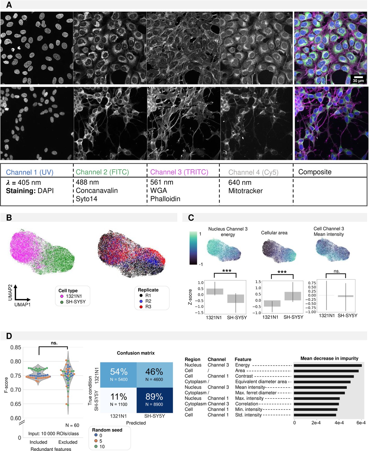
Shallow classification using manually defined features.
(A) Image overview of 1321N1 (top) and SH-SY5Y (bottom) cells after cell painting (CP) staining acquired at higher magnification (Plan Apo VC 60xA WI DIC N2, NA = 1.20). Scale bar is 30 µm. The channel, wavelength, and dye combination used is listed in the table below the figure. This color code and channel numbering is used consistently across all figures. (B) UMAP dimensionality reduction using handcrafted features. Each dot represents a single cell. The colour reflects either cell type condition (left) or replicate (right). This shows that UMAP clustering is a result of cell type differences and not variability between replicates. (C) Feature importance deducted from the UMAP (feature maps). Each dot represents a single cell. Three exemplary feature maps are highlighted alongside the quantification per cell type. These feature representations help understand the morphological features that underlie the cluster separation in UMAP. (D) Random Forest classification performance on the manually defined feature data frame with and without exclusion of redundant features. Average confusion matrix (with redundant features) and Mean Decrease in Impurity (reflecting how often this feature is used in decision tree splits across all random forest trees). All features used in the UMAP are used for random forest (RF) building. Each dot in the violinplot represents the F-score of one classifier (model initialisation, N=30). Classifiers were trained 10 x with three different random seeds.
Figure 1—figure supplement 1

PCA dimensionality reduction on handcrafted features extracted from monocultures of 1321N1 and SH-SY5Y cells.
Each point represents an individual cell.
Figure 2 with 1 supplement
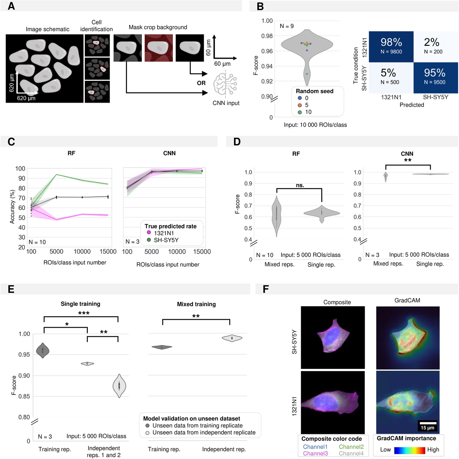
Convolutional neural network classification of monoculture conditions.
(A) Schematic of image pre-processing for convolutional neuronal network (CNN) classification. (B) CNN accuracy and confusion matrix on cell type classification in monocultures. Each dot in the violinplot represents the F-score of one classifier (model initialisations, N=9). (C) Shallow vs. deep learning accuracy for a varying number of input instances (region of interests, ROIs). Each dot in the violinplot represents the F-score of one classifier (model initialisation, N). The ribbon represents the standard deviation on the classifiers. (D) The impact of experimental variability in the training dataset on model performance for shallow vs. deep learning. Classifiers were trained on either 1 (single rep.) or multiple (mixed reps.) replicates (where each replicate consists of a new biological experiment). Mann-Whitney-U-test, p-values resp. 0.7304 and 0.000197. Each violinplot represents the F-score of N classifiers (model initialisations). (E) The performance of deep learning classifiers trained in panel D on single replicates (low variability) or mixed replicates (high variability) on unseen images from either the training replicate (cross-validation) or an independent replicate (independent testing) (where each replicate consists of a new biological experiment). Kruskal-Wallis test on single training condition, p-value of 0.026 with post-hoc Tukey test. Mann-Whitney-U-test on mixed training, p-value of 7.47e-6. Each violinplot represents the F-score of one classifier (model initialisation, N=3). (F) Images of example inputs given to the CNN. The composite image contains an overlay of all cell painting (CP) channels (left). The GradCAM image overlays the GradCAM heatmap on top of the composite image, highlighting the most important regions according to the CNN (right). One example is given per cell type.
Figure 2—figure supplement 1
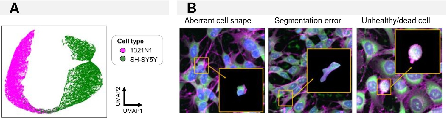
Cell classification in monoculture conditions.
(A) UMAP of feature embeddings of the convolutional neuronal network (CNN) trained to classify 1321N1 and SH-SY5Y monocultures. Each point represents an individual cell. (B) Examples of misclassified region of interests (ROIs).
Figure 3 with 1 supplement
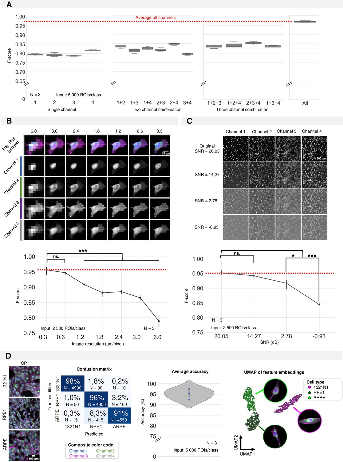
Required input quality for cell type classification.
(A) Performance of the convolutional neuronal network (CNN) when only a selection of image channels is given as training input. Each boxplot represents the F-score of one classifier (model initialisation, N=3). Channel numbering is in accordance with Figure 1A. (1=DAPI; 2=FITC; 3=Cy3; 4=Cy5) (B) Simulation of the effect of increased pixel size (reduced spatial resolution) on the classification performance. Each point is the average of three CNN model initializations (N), with bars indicating the standard deviation between models. Red line indicates the average F-score of the original crops. (C) Simulation of the effect of added Gaussian noise (reduced signal-to-noise ratio) on the classification performance. Each point is the average of three CNN model initialisations, with bars indicating the standard deviation between models. Red line indicates the average F-score of the original images. Statistics were performed using a Kruskal-Wallis test with post-hoc Tukey test. (D) CNN performance on 1321N1, RPE1, and ARPE cells. Dots represent different model initialisations (N=3).
Figure 3—figure supplement 1
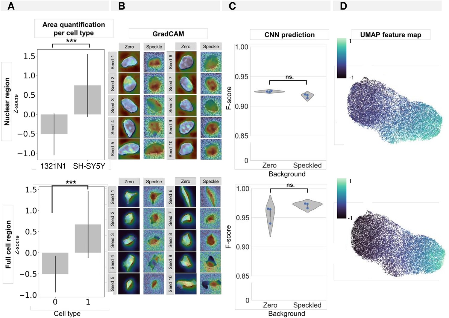
Influence of the nuclear/cellular size on convolutional neuronal network (CNN) prediction and association with the input background (space artificially set to zero outside of the segmentation mask).
(A) Quantification of average nuclear/cellular size per cell type. (B) GradCAM images for 10 random seeds for crops and CNN models trained with background either set to zero or ‘random speckle.’ (C) CNN prediction results for models trained on crops with background either set to zero or ‘random speckle.’ Each dot in the violinplots represents the F-score of one classifier (model initialisation, N=3). (D) Feature map (see UMAP in Figure 1B and C) of 1321N1 and SH-SY5Y cells showing the contribution of nuclear/cellular area to the cell type cluster separation. Each point represents an individual cell.
Figure 4 with 8 supplements
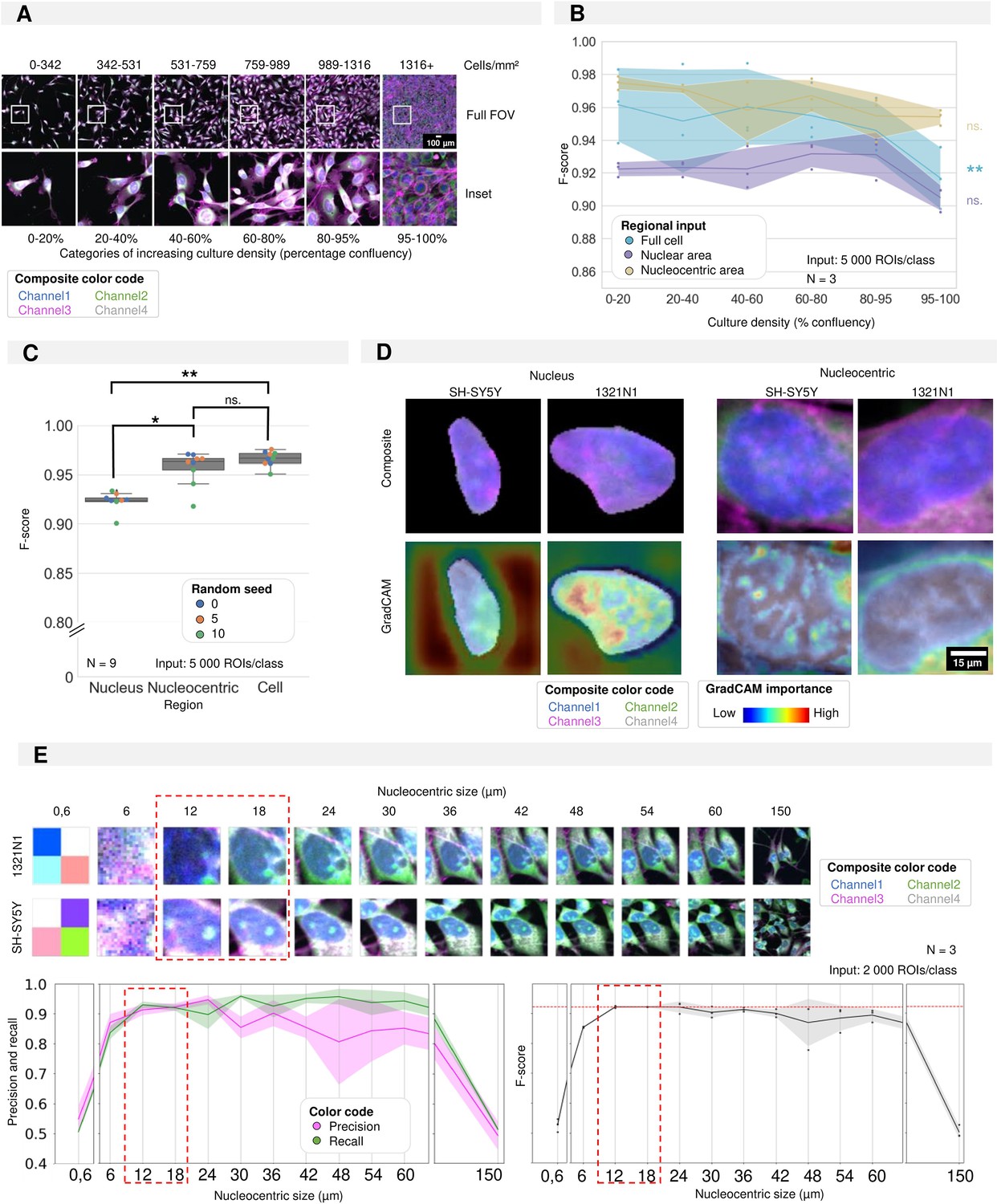
Required regional input for accurate convolutional neuronal network (CNN) training in cultures of high density.
(A) Selected images and insets for increasing culture density with the density categories used for CNN training. (B) Results of three CNN models trained using different regional inputs (the full cell, only nucleus, or nucleocentric area) and evaluated on data subsets with increasing density. Each dot represents the F-score of one classifier (model initialisation, N=3) tested on a density subset. Classifiers were trained with the same random seed. Ribbon represents the standard deviation. (C) CNN performance (F-score) of CNN models using different regional inputs (full cell, only nucleus, or nucleocentric area). Each boxplot represents three model initialisations for three different random seeds (N=9). (D) Images of example inputs for both the nuclear and nucleocentric regions. The composite image contains an overlay of all cell painting (CP) channels (top). The GradCAM image overlays the GradCAM heatmap on top of the composite image, highlighting the most important regions according to the CNN (bottom). One example is given per cell type. (E) Systematic in- and decrease (default of 18 µm used in previous panels) of the patch size surrounding the nuclear centroid used to determine the nucleocentric area. Each dot represents the results of one classifier (model initialisation, N=3). Ribbon represents the standard deviation. The analysis was performed using a mixed culture dataset of 1321N1 and SH-SY5Y cells (Figure 5).
Figure 4—figure supplement 1
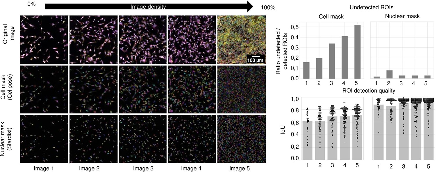
Segmentation performance as a function of cell density.
Left: Representative images of 1321N1 cells with increasing density alongside their cell and nuclear mask produced using resp. Cellpose and Stardist. Images are numbered from 1 to 5 with increasing density. Upper right: The number of region of interests (ROIs) detected in comparison to the ground truth (manual segmentation). A ROI was considered undetected when the intersection over union (IoU) was below 0.15. Each bar refers to the image number on the left. The IoU quantifies the overlap between ground truth (manually segmented ROI) and the ROI detected by the segmentation algorithm. It is defined as the area of the overlapping region over the total area. IoU for increasing cell density for cell and nuclear masks is given in the bottom right. Each point represents an individual ROI. Each bar refers to the image number on the left.
Figure 4—figure supplement 2
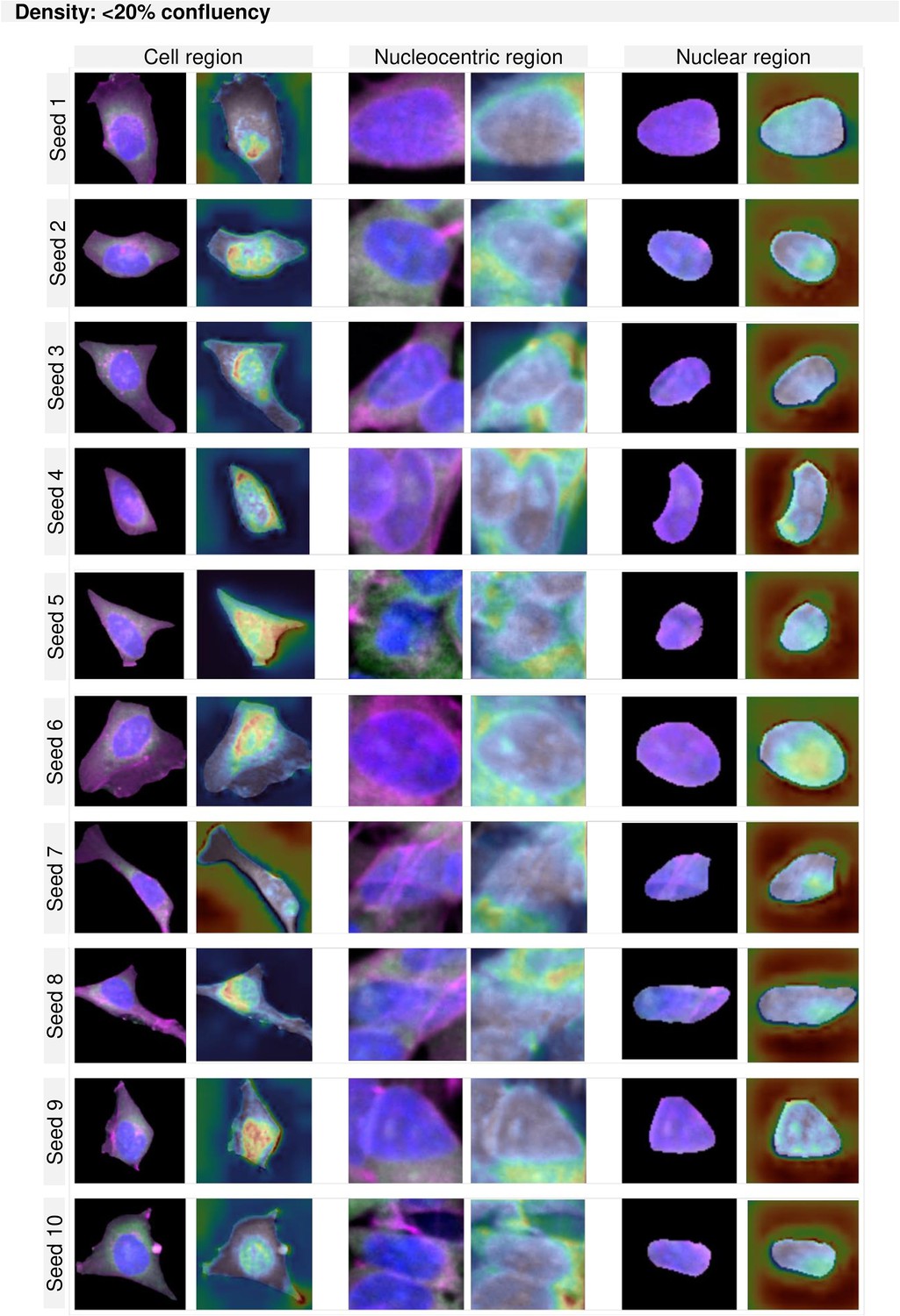
GradCAM maps per region and density for cultures of less than 20% confluency.
Figure 4—figure supplement 3
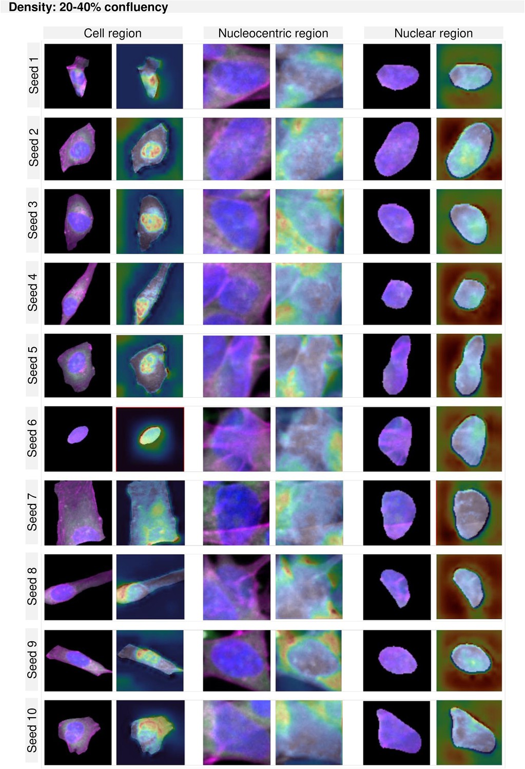
GradCAM maps per region and density for cultures between 20–40% confluency.
Figure 4—figure supplement 4
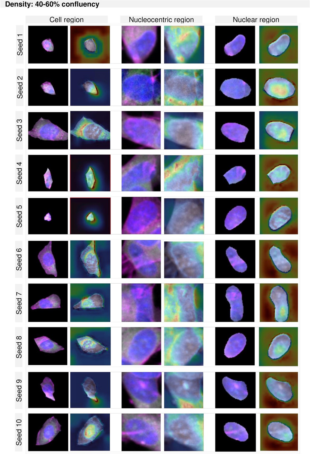
GradCAM maps per region and density for cultures between 40–60% confluency.
Figure 4—figure supplement 5
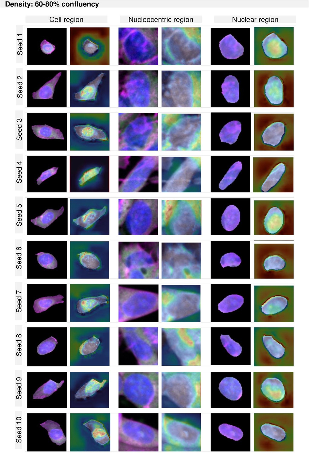
GradCAM maps per region and density for cultures between 60–80% confluency.
Figure 4—figure supplement 6
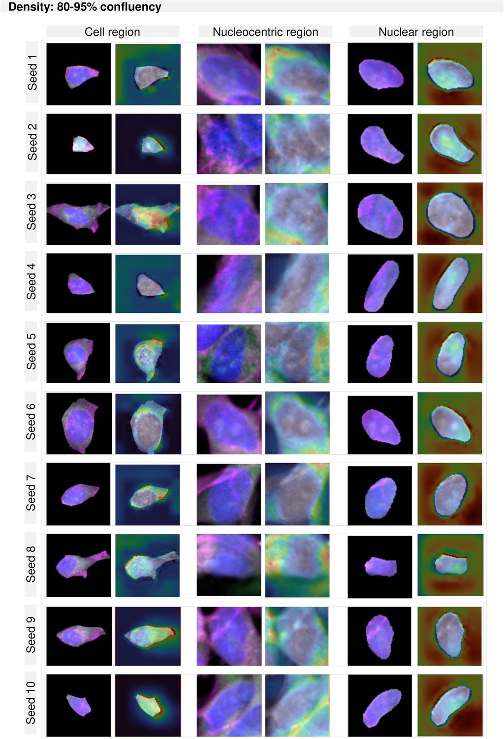
GradCAM maps per region and density for cultures between 80–95% confluency.
Figure 4—figure supplement 7
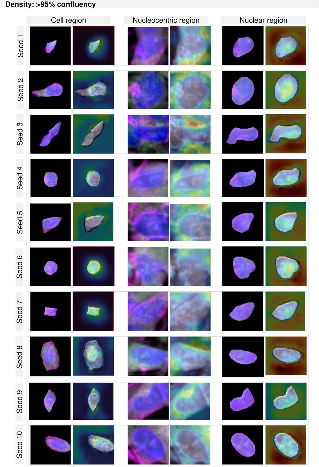
GradCAM maps per region and density for cultures higher than 95% confluency.
Figure 4—figure supplement 8
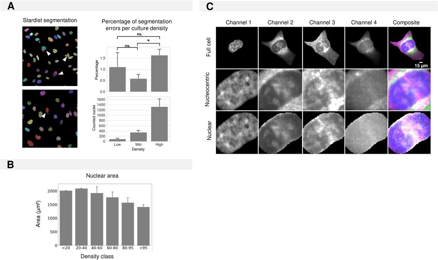
Required regional input for CNN training in cultures of increasing density.
(A) Examples of segmentation mistakes made by the Stardist segmentation algorithm for nuclear segmentation for different culture densities. (B) Nuclear area in function of density. (C) Definition of cell regions given as training input for nuclear and nucleocentric model training.
Figure 5 with 2 supplements
Cell type prediction in mixed cultures by post-hoc ground truth identification.
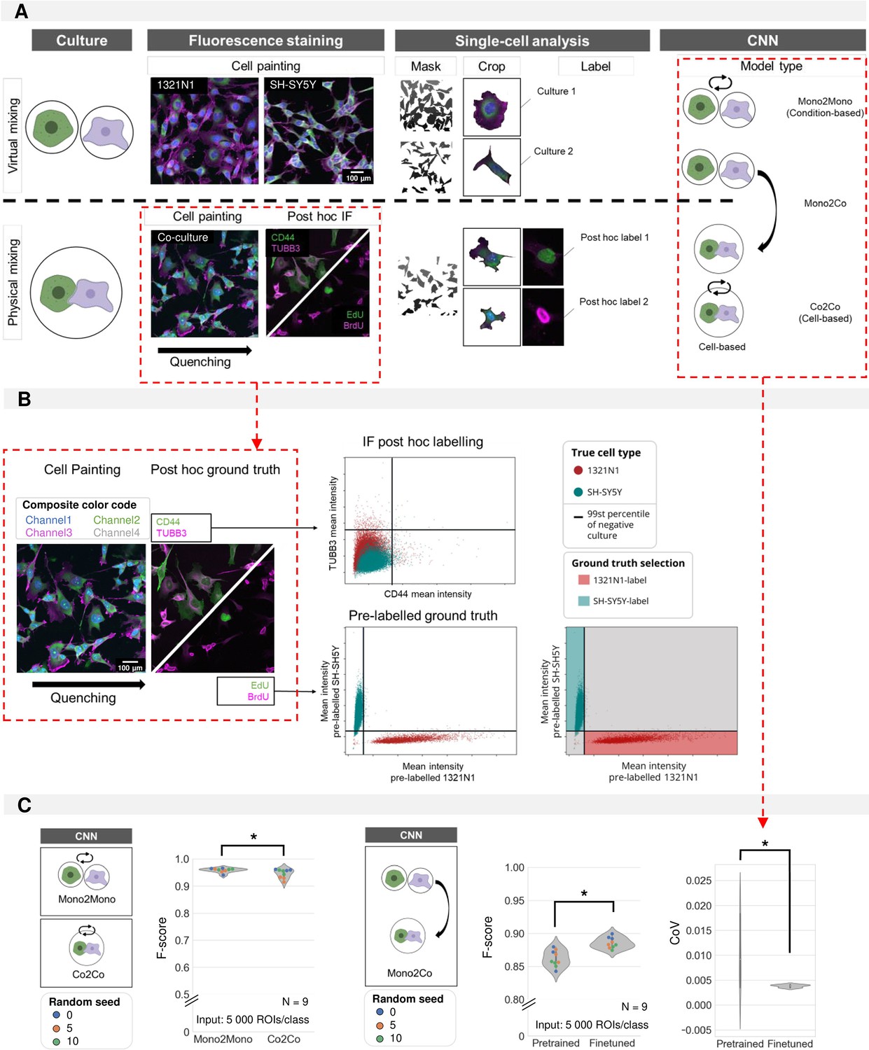
(A) Schematic overview of virtual vs. physically mixed cultures and the subsequent convolutional neuronal network (CNN) models. For virtual mixing, individual cell types arise from distinct cultures, the cell type label was assigned based on the culture condition. For physical mixing, the true phenotype of each crop was determined by intensity thresholding after post-hoc staining. Three model types are defined: Mono2Mono (culture-based label), Co2Co (cell-based label), and Mono2Co (trained with culture-based label and tested on cell-based label). (B) Determining ground-truth phenotype by intensity thresholding on immunofluorescence staining (IF) (top) or pre-label (bottom). The threshold was determined on the intensity of monocultures. Only the pre-labelled ground-truth resulted in good cell type separation by thresholding for 1321N1 vs. SH-SY5Y cells. (C) Mono2Mono (culture-based ground truth) vs. Co2Co (cell-based ground truth) models for cell type classification. Analysis performed with full cell segmentation. Mann-Whitney-U-test p-value 0.0027. Monoculture-trained models were tested on mixed cultures. Pretrained models were trained on independent biological replicates. These could be finetuned by additional training on monoculture images from the same replicate as the coculture. This was shown to reduce the variation between model iterations (Median performance: Mann-Whitney-U-test, p-value 0.0015; Coefficient of variation: Mann-Whitney-U-test, p-value 3.48e-4). Each dot in the violinplots represents the F-score of one classifier (model initialisation, N=9). Classifiers were trained 3 x with three different random seeds.
Figure 5—figure supplement 1
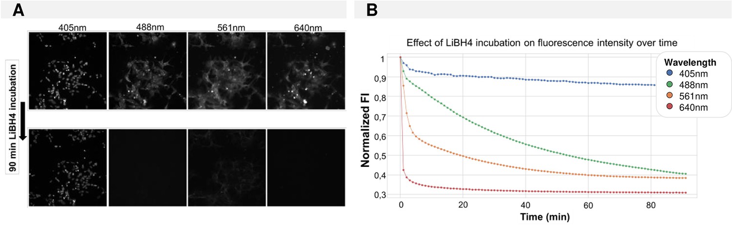
Fluorescence quenching over time using LiBH4.
(A) Images before and after quenching for all four fluorescence channels. (B) Time curve of normalized image-level fluorescence intensity during incubation with 1 mg/ml LiBH4.
Figure 5—figure supplement 2
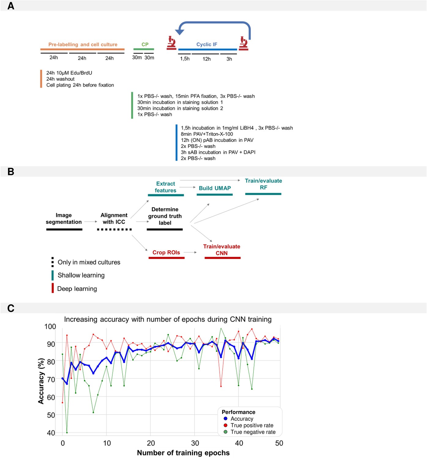
Methods.
(A) Pipeline used for morphological profiling in mixed cultures. (B) Overview of the steps within the image analysis pipeline. (C) Evaluation of accuracy, true negative, and true positive rate during convolutional neuronal network (CNN) training (1321N1 vs. SH-SY5Y in monocultures) across all 50 epochs.
Figure 6
Induced pluripotent stem cell (iPSC)-derived differentiation staging using morphology profiling.
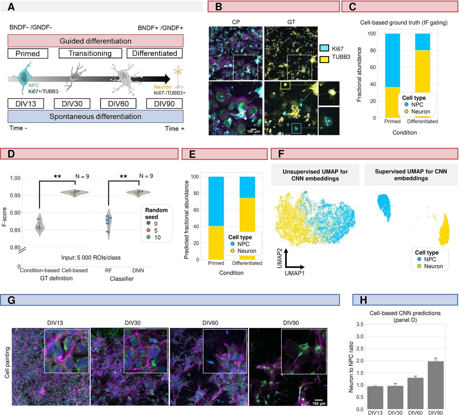
(A) Schematic overview of guided vs. spontaneous neural differentiation. DIV = days in vitro. Selected timepoints for analysis of the spontaneously differentiation culture were 13, 30, 60, and 90 d from the start of differentiation of iPSCs. (B) Representative images of morphological staining (colour code as defined in Figure 1A) and post-hoc immunofluorescence staining (IF) of primed and differentiated iPSC-derived cultures (guided differentiation). Ground-truth determination is performed using TUBB3 (for mature neurons) and Ki67 (mitotic progenitors). (C) Fraction of neurons vs. neural progenitor (NPC) cells in the primed vs. differentiated condition as determined by IF staining. Upon guided differentiation, the fraction of neurons increased. (D) Left: CNN performance when classifying neurons (Ki67-/TUBB3+) vs. NPC (Ki67+/TUBB3-) cells using either a condition-based or cell-type-based ground truth. Each dot in the violinplots represents the F-score of one classifier (model initialisation). Classifiers were trained with different random seeds. Mann-Whitney-U-test, p-value 4.04e-4. Right: comparison of CNN vs. RF performance. Mann-Whitney-U-test, p-value 2.78e-4. (E) Fractional abundance of predicted cell phenotypes (NPC vs. neurons) in primed vs. differentiated culture conditions using the cell-based CNN. (F) Unsupervised and supervised UMAP of the cell-based CNN feature embeddings. Plot colour-coded by cell type. Points represent individual cells. (G) Representative images of spontaneously differentiating neural cultures. Colour code as defined in Figure 1A. (H) Prediction of differentiation status using the cell-based CNN model trained on guided differentiated culture.
Figure 7
Induced pluripotent stem cell (iPSC) cell type identification using morphology profiling.
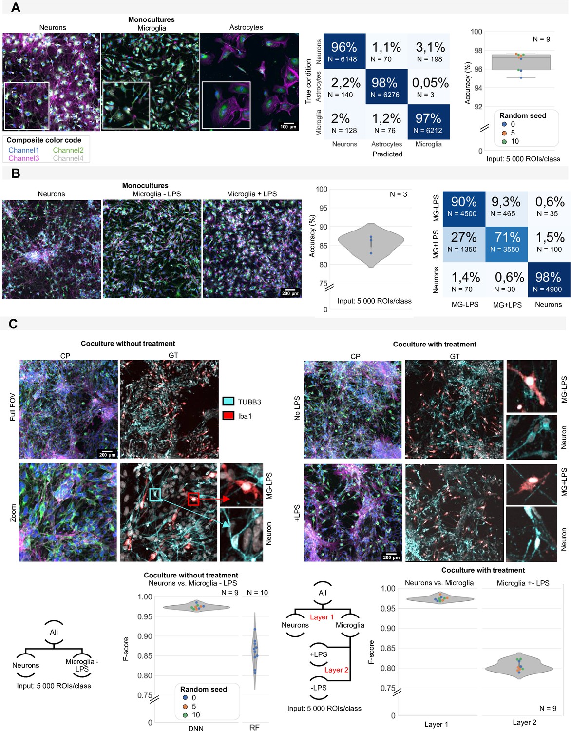
(A) Representative images of iPSC-derived neurons, astrocytes, and microglia in monoculture with morphological staining. Colour code as defined in Figure 1A. Prediction accuracy of a convolutional neuronal network (CNN) trained to classify monocultures of iPSC-derived astrocytes, microglia, and neurons with confusion matrix (average of all models). Each dot in the boxplot represents the F-score of one classifier (model initialisation, N=9). Classifiers were trained 3 x with three different random seeds. (B) Representative images of monocultures of iPSC-derived neurons and microglia treated with LPS or control. Colour code as defined in Figure 1A. Prediction accuracy and confusion matrix (average of all models) are given. Each dot in the violinplot represents the F-score of one classifier (model initialisation, N=3). (C) Representative images of a mixed culture of iPSC-derived microglia and neurons. Ground-truth identification was performed using immunofluorescence staining (IF). Each dot in the violinplot represents the F-score of one classifier (model initialisation). Classifiers were trained three different random seeds. Results of the CNN are compared to shallow learning (random forest, RF). The same analysis was performed for mixed cultures of neurons and microglia with LPS treatment or control. A layered approach was used where first the neurons were separated from the microglia before classifying treated vs. non-treated microglia. Each dot in the violinplot represents the F-score of one classifier (model initialisation, N=9). Classifiers were trained 3 x with three different random seeds.
Tables
Table 1
Definition of handcrafted features (according to the scikit-image documentation).
All of these features were extracted for each fluorescent channel (1-4) and region (nucleus, cytoplasm, and whole-cell) in the cell painting images.
| Feature name | Description | Category |
|---|---|---|
| Intensity max | Maximal pixel intensity inside the ROI | Intensity |
| Intensity mean | Mean pixel intensity inside the ROI | Intensity |
| Intensity min | Minimal pixel intensity inside the ROI | Intensity |
| Intensity Std | Standard deviation of the pixel intensities inside the ROI | Intensity |
| Area | Area of the ROI | Shape |
| Area convex | The area of the convex polygon that encloses the ROI | Shape |
| Area filled | Area of the ROI including all holes inside the ROI | Shape |
| Axis major length | The length of the major axis of the ellipse that has the same normalized second central moments as the region. | Shape |
| Axis minor length | The length of the minor axis of the ellipse that has the same normalized second central moments as the region. | Shape |
| Centroid | Coordinates of the center of the ROI | Shape |
| Eccentricity | Eccentricity of the ellipse that has the same second-moments as the ROI. | Shape |
| Equivalent diameter area | The diameter of a circle with the same area as the ROI. | Shape |
| Extent | The ratio of the Area of the ROI to the Area of the bounding box around the ROI. | Shape |
| Feret diameter max | The longest distance between points around a ROIs’ convex polygon. | Shape |
| Orientation | The angle between the X-axis and the major axis. | Shape |
| Perimeter | Length of the contour of the ROI | Shape |
| Perimeter crofton | Perimeter of the ROI approximated by the Crofton formula in four directions. | Shape |
| Solidity | The ratio of the number of pixels inside the ROI to the number of pixels of the convex polygon. | Shape |
| Contrast | The difference between the maximum intensity and minimum intensity pixel inside the ROI. | Texture |
| Dissimilarity | The average difference in pixel intensity between neighbouring pixels. | Texture |
| Homogeneity | Value for similarity of pixels in the ROI. | Texture |
| Energy | Value for the local change of pixel intensities in the ROI. | Texture |
| Correlation | Value for the linear dependency of pixels in the ROI. | Texture |
| ASM (angular second moment) | Value for the uniformity of pixel values in a ROI. | Texture |
Table 2
Specifications of morphological staining composition.
| Staining solution 1 | |||||||
|---|---|---|---|---|---|---|---|
| Dye | Target | Excitation (nm) | Emission (nm) | Stock concentration | End dilution | Supplier | Catalog # |
| DAPI | Nucleus | 350 | 470 | 2.5 mg/ml | 1/500 | Sigma Aldrich | D9542 |
| Concanavalin | ER | 480 | 490–540 | 5 mg/ml | 1/300 | Life Technologies | C11252 |
| WGA | Golgi | 550 | 560–570 | 1 mg/ml | 1/600 | Life Technologies | W32464 |
| Phalloidin | Actin | 570 | 580–610 | 66 µM | 1/1000 | Life Technologies | A12380 |
| Mitotracker | Mitochondria | 640 | 650–660 | 1 mM | 1/1000 | Life Technologies | M22426 |
| Staining solution 2 | |||||||
| Syto14 | Nucleoli/RNA | 525 | 540–580 | 5 mM | 1/1000 | Life Technologies | S7576 |
Table 3
Used antibodies.
| Antibody | Host | Supplier | Catalog # | RRID | |
|---|---|---|---|---|---|
| Primary antibodies | Anti-BrdU | Sheep | Abcam | ab1893 | AB_302659 |
| Anti-MAP2 | Chicken | Synaptic systems | 188006 | AB_2619881 | |
| Anti-TUBB3 | Mouse | BioLegend | 801202 | AB_2313773 | |
| Anti-CD44 | Mouse | Millipore | MAB4065 | AB_95019 | |
| Anti-GFAP | Goat | Abcam | ab53554 | AB_880202 | |
| Anti-Iba1 | Rabbit | Wako | 019–19741 | AB_839504 | |
| Anti-Ki67 | Rabbit | Abcam | ab15580 | AB_443209 | |
| Secondary antibodies | Anti-mouse-Cy3 | Donkey | Jackson ImmunoResearch | 715-165-150 | AB_2340813 |
| Anti-mouse-Cy5 | Donkey | Jackson ImmunoResearch | 715-175-150 | AB_2340819 | |
| Anti-sheep-Cy3 | Donkey | Jackson ImmunoResearch | 713-165-147 | AB_2315778 | |
| Anti-sheep-Cy5 | Donkey | Jackson ImmunoResearch | 713-175-147 | AB_2340730 | |
| Anti-chicken-Cy5 | Donkey | Jackson ImmunoResearch | 703-175-155 | AB_2340365 | |
| Anti-goat-Cy3 | Donkey | Jackson ImmunoResearch | 705-165-147 | AB_2307351 | |
| Anti-Guinea pig-Cy3 | Donkey | Jackson ImmunoResearch | 706-165-148 | AB_2340460 | |
| Anti-Rabbit-Cy5 | Donkey | Jackson ImmunoResearch | 711-175-152 | AB_2340607 | |
Table 4
Specifications of the used laser lines, excitation, and emission filters.
Channel dimension | Laser line (nm) | Excitation filter (nm) | Emission filter (nm) |
|---|---|---|---|
| Channel 1 | 405 | Di01-T405/488/568/647−13x15 × 0.5 | B447/60 |
| Channel 2 | 488 | B520/35 | |
| Channel 3 | 561 | B617/73 | |
| Channel 4 | 640 | B685/40 |
Table 5
Python packages used for image and data analysis alongside the software version.
| Package | Version | Reference |
|---|---|---|
| pathlib | 1.0.1 | |
| numpy | 1.21.2 | Harris et al., 2020 |
| tifffile | 2021.7.2 | |
| pytorch | 1.13.0 | Paszke et al., 2019 |
| torchvision | 0.14.0 | |
| nd2reader | 3.3.0 | |
| matplotlib | 3.5.2 | Hunter, 2007 |
| scikit-image | 0.19.3 | Van der Walt et al., 2014 |
| scikit-learn | 1.1.3 | Pedregosa et al., 2011 |
| argparse | 1.4.0 | |
| cellpose | 2.1.1 | Stringer et al., 2021 |
| tqdm | 4.64.1 | |
| scipy | 1.9.3 | Virtanen et al., 2020 |
| pandas | 1.5.1 | McKinney, 2010 |
| seaborn | 0.12.1 | Waskom et al., 2022 |
| imbalanced-learn | 0.10.0 | Lemaître et al., 2017 |
| StarDist | 0.8.5 | Weigert et al., 2020 |
Additional files
Download links
A two-part list of links to download the article, or parts of the article, in various formats.
Downloads (link to download the article as PDF)
Open citations (links to open the citations from this article in various online reference manager services)
Cite this article (links to download the citations from this article in formats compatible with various reference manager tools)
Unbiased identification of cell identity in dense mixed neural cultures
eLife 13:RP95273.
https://doi.org/10.7554/eLife.95273.4


