Figures and data in Balancing reaction-diffusion network for cell polarization pattern with stability and asymmetry

Figures
Tables
Additional files

12 figures, 4 tables and 3 additional files

Figures

Figure 1 with 6 supplements

Download asset Open asset

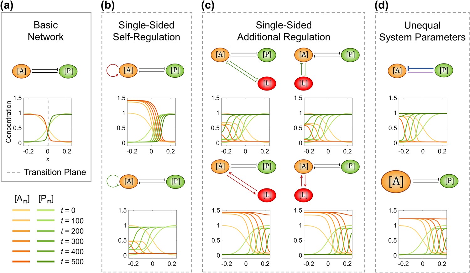
The single modification on the antagonistic 2-node network causes the collapse of cell polarization pattern.

(a) Basic network with the transition plane (mid-plane) marked by gray dashed line. (b) Two subtypes of single-sided self-regulation. (c) Four subtypes of single-sided additional regulation. The corresponding spatial concentration distribution of $[L_{m}]$ at $t = 0, 100, 200, 300, 400, a n d 500$ , and the subtle difference between left and right panels are detailed in Figure 1—figure supplement 3. (d) Two subtypes of unequal system parameters, exemplified by unequal inhibition intensity and unequal cytoplasmic concentration. For each network, the corresponding spatial concentration distribution of $[A_{m}]$ and $[P_{m}]$ at $t = 0, 100, 200, 300, 400, a n d 500$ are shown beneath with a color scheme listed in the bottom left corner. Note that within a network, normal arrows and blunt arrows symbolize activation and inhibition respectively.

Figure 1—figure supplement 1

Download asset Open asset

The initial state at $t = 0$ (shown on the left) and stable state at $t = 500$ (shown in the middle) of the cell polarization pattern generated by the simple 2-node network and C. *elegans* 5-node network (shown on the right).

Note that the spatial concentration distribution on the cell membrane ( $[X_{m}] (x, 0)$ ) is averaged over all established viable parameter sets for each molecular species (*i.e*., 122 among 5,151 sets, ~2.37%, for the simple 2-node network; 602 among 262,701 sets, ~0.229%, for the *C. elegans* 5-node network). Note that within a network, normal arrows and blunt arrows symbolize activation and inhibition respectively.

Figure 1—figure supplement 2

Download asset Open asset

The antagonistic 2-node network initiated with different initial spatial concentration distributions on the cell membrane.

(a) Uniform initial distribution with a higher global concentration in $[A]$ than $[P]$ . (b) Uniform initial distribution with a higher global concentration in $[P]$ than $[A]$ . (c) Polarized initial distribution with a posterior shift in the transition plane of $[P]$ . (d) Polarized initial distribution with a posterior shift in the transition planes of $[A]$ and $[P]$ . (e) Polarized initial distribution with symmetric curve shapes for [A] and [P], where their concentrations in the anterior and posterior are slightly different. (f) Polarized initial distribution with asymmetric curve shapes for $[A]$ and $[P]$ , where their concentrations in the anterior are almost the same. (g) Polarized initial distribution with asymmetric curve shapes for $[A]$ and $[P]$ , where the widths of their transition regions are different. (h) Gaussian noise distribution for $[A]$ and $[P]$ . For each simulation, the corresponding spatial concentration distribution of $[A_{m}]$ and $[P_{m}]$ at $t = 0, 100, 200, 300, 400, a n d 500$ are shown with a color scheme listed in the bottom right corner. Note that within a simulation, the mathematical expressions for the initial distributions are described on top (upper: $[A_{m}]$ ; lower: $[P_{m}]$ ; $N (μ, σ)$ : Gaussian noise distribution with a mean of μ and a standard deviation of $σ$ ).

Figure 1—figure supplement 3

Download asset Open asset

The antagonistic 2-node network added with four subtypes of single-sided additional regulation (corresponding to Figure 1c) causes the collapse of cell polarization pattern.

The node $[L]$ is added anteriorly or posteriorly, mutually activating or inhibiting the existing anterior node $[A]$ (1^st row). For each network, the corresponding spatial concentration distribution of $[A_{m}]$ (2^nd row), $[P_{m}]$ (3^rd row), and $[L_{m}]$ (4^th row) at $t = 0, 100, 200, 300, 400, a n d 500$ are shown beneath with a color scheme listed in the bottom right corner. Note that within a network, normal arrows and blunt arrows symbolize activation and inhibition respectively.

Figure 1—figure supplement 4

Download asset Open asset

With different initial spatial concentration distributions on the cell membrane, the single modification on the antagonistic 2-node network causes the collapse of cell polarization pattern.

Initial distributions are shown in the 1^st column, which are the same as those shown in Figure 1—figure supplement 2d (2^nd row), Figure 1—figure supplement 2e (3^rd row), and Figure 1—figure supplement 2g (4^th row), alongside the basic network (2^nd column) and the ones added with single-sided self-regulation (exemplified by self-activation on $[A]$ , where $q_{A 1}^{A} = 1$ and $q_{A 2}^{A} = 0.012$ , 3^rd column), single-sided additional regulation (exemplified by $[A]$ ~ $[L]$ mutual inhibition with $[L]$ in the posterior, where $γ_{L} = α_{L} = 0.05$ , $k_{L 1}^{A} = k_{A 1}^{L} = 0.05$ , and $k_{L 2}^{A} = k_{A 2}^{L} = 0.025$ , 4^th column), and unequal system parameters (exemplified by unequal inhibition intensity, where $k_{P 2}^{A}$ is increased from 1 to 1.6, 5^th column; exemplified by unequal cytoplasmic concentration, where $[A_{c}]$ is increased from 1 to 1.25, 6^th column) shown on top. For each network, the corresponding spatial concentration distribution of $[A_{m}]$ , $[P_{m}]$ , and $[L_{m}]$ at $t = 0, 100, 200, 300, 400, a n d 500$ are shown beneath with a color scheme listed in the bottom right corner. Note that within a network, normal arrows and blunt arrows symbolize activation and inhibition respectively. Note that within a simulation, the mathematical expressions for the initial distributions are described on the left (upper: $[A_{m}]$ ; lower: $[P_{m}]$ ).

Figure 1—figure supplement 5

Download asset Open asset

With parameters (*i.e.*, $γ$ , $α$ , $k_{1}$ , $k_{2}$ , $q_{1}$ , $q_{2}$ , and $[X_{c}]$ ) assigned with various values concerning all nodes and regulations (detailed in Appendix 1—table 2, Appendix 1—table 3), the single modification on the simple 2-node network (top panel) and *C. elegans* 5-node network (bottom panel) causes the collapse of cell polarization pattern.

(a) Basic network with the transition plane marked by gray dashed line. (b) Two subtypes of single-sided regulation. For a 2-node network, a self-activation ( $q_{A 1}^{A} = 1$ and $q_{A 2}^{A} = 0.025$ , 2^nd column) or anteroposterior mutual inhibition ( $γ_{L} = α_{L} = 0.02$ , $k_{L 1}^{A} = k_{A 1}^{L} = 1$ , $k_{L 2}^{A} = k_{A 2}^{L} = 2$ , and $[L_{c}] = 1$ , 3^rd column) is added on the node $[A]$ . For a 5-node network, anteroposterior mutual inhibition between $[A]$ and $[L]$ (2^nd column) or anterior mutual activation between $[A]$ and $[C]$ (3^rd column) is eliminated. (c) Two subtypes of unequal system parameters, exemplified by unequal inhibition intensity and unequal cytoplasmic concentration. For a 2-node network, the inhibition intensity $k_{P 2}^{A}$ is increased from 3.8471 to 5 (4^th column); the cytoplasmic concentration $[A_{c}]$ is increased from 1.5361 to 2 (5^th column). For a 5-node network, the inhibition intensity $k_{L 2}^{A}$ is increased from 3.7357 to 15 (4^th column); the cytoplasmic concentration $[L_{c}]$ is increased from 2.3793 to 5 (5^th column). For each network, the corresponding spatial concentration distribution of $[A_{m}]$ , $[C_{m}]$ , $[P_{m}]$ , $[L_{m}]$ , and $[H_{m}]$ at $t = 0, 100, 200, 300, 400, a n d 500$ are shown beneath with a color scheme listed in the bottom right corner. Note that within a network, normal arrows and blunt arrows symbolize activation and inhibition respectively.

Figure 1—video 1

Download asset

posterframe for video — The spatial concentration distribution of each molecular species on the cell membrane over time generated by the antagonistic 2-node network and the ones with a single modification added, corresponding to Figure 1.

Figure 2 with 1 supplement

Download asset Open asset

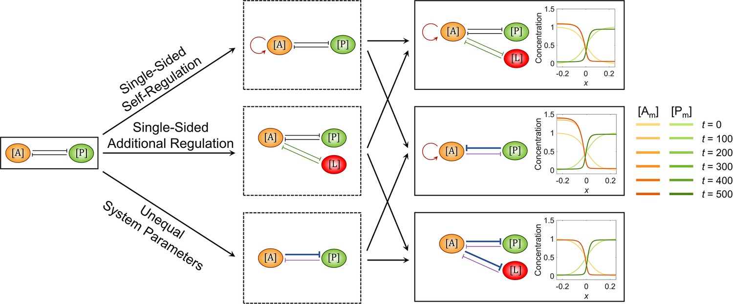
The combination of two opposite modifications recovers the cell polarization pattern stability.

The basic network and the ones added with a single modification are shown in the 1^st and 2^nd columns, respectively; the three combinatorial networks composed of any two of the three single modifications are shown in the 3^rd column. For each network, the corresponding spatial concentration distribution of $[A_{m}]$ and $[P_{m}]$ at $t = 0, 100, 200, 300, 400, a n d 500$ are shown beneath with a color scheme listed on the right. Here, the value assignments on the modifications in the 3^rd column are as follows: $q_{A 2}^{A} = 0.012$ and $k_{L 2}^{A} & k_{A 2}^{L} = 0.01$ for 1^st row, $q_{A 2}^{A} = 0.012$ and $k_{P 2}^{A} = 1.24$ for 2^nd row, and $q_{A 2}^{A} = 0.012$ and $k_{A 2}^{P} & k_{A 2}^{L} = 2$ for 3^rd row. Note that within a network, normal arrows and blunt arrows symbolize activation and inhibition respectively.

Figure 2—video 1

Download asset

Figure 3

Download asset Open asset

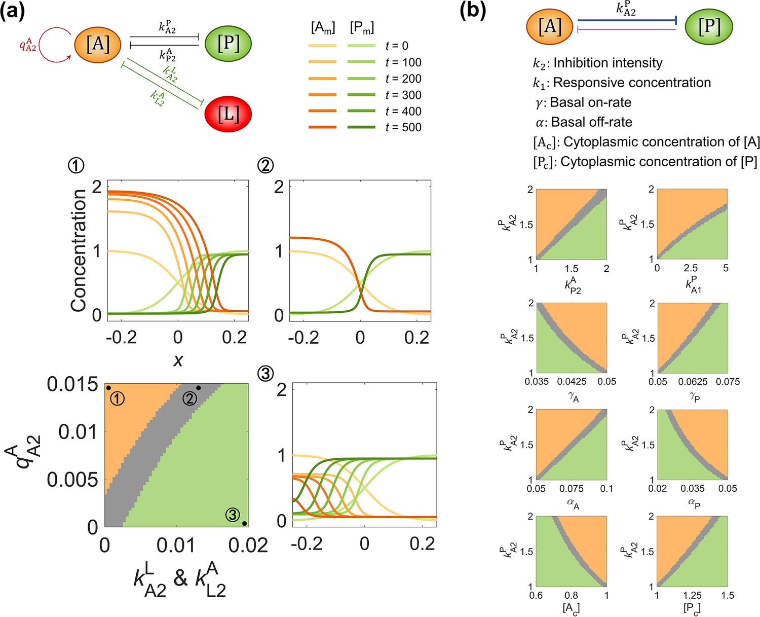
The balance between system parameters is needed for maintaining pattern stability.

(a) The phase diagram between $q_{A 2}^{A}$ and $k_{L 2}^{A} & k_{A 2}^{L}$ in the network modified by self-activation (quantified by $q_{A 2}^{A}$ ) and additional inhibition (quantified by $k_{L 2}^{A} & k_{A 2}^{L}$ ) on $[A]$ . The representative parameter assignment for each phase is marked with ① (*i.e.*, $q_{A 2}^{A} = 0.015$ and $k_{L 2}^{A} & k_{A 2}^{L} = 0$ with a homogeneous state dominated by $[A]$ ), ② (*i.e.*, $q_{A 2}^{A} = 0.015$ and $k_{L 2}^{A} & k_{A 2}^{L} = 0.0135$ with a stable polarized state), and ③ (*i.e.*, $q_{A 2}^{A} = 0.02$ and $k_{L 2}^{A} & k_{A 2}^{L} = 0$ with a homogeneous state dominated by $[P]$ ). The corresponding spatial concentration distribution of $[A_{m}]$ and $[P_{m}]$ at $t = 0, 100, 200, 300, 400, a n d 500$ are shown around the phase diagram with a color scheme listed on top. (b) The phase diagram between responsive concentration $k_{1}$ , basal on-rate $γ$ , basal off-rate $α$ , cytoplasmic concentration $[X_{c}]$ , and inhibition intensity $k_{2}$ . For each phase diagram in (a) (b), the final state dominated by $[A]$ or $[P]$ or stably polarized is colored in orange, green, and gray, respectively. Note that within a network, normal arrows and blunt arrows symbolize activation and inhibition respectively.

Figure 4 with 1 supplement

Download asset Open asset

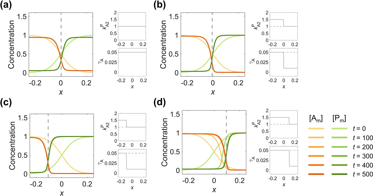
Adopting parameter sets corresponding to opposite interface velocities on two sides of the interface, the zero-velocity interface position of the polarity pattern is shiftable and regulatable.

(a) Spatially inhomogeneous parameters (2^nd column) of a symmetric 2-node network generate a symmetric pattern (1^st column), from the same simulation in Figure 1a. (b) Using the parameter combination with the posterior-shifting interface on the left and anterior-shifting interface on the right, a stable polarity pattern (1^st column) can be remained by increasing $k_{A 2}^{P}$ to 1.5 at $x < 0$ and decreasing $γ_{A}$ to 0.01 at (2^nd column). (**c–d**) The stable interface position can be optionally adjusted by setting the change position of the step-up function (2^nd column). (c) As in (b), but changing the step position to $x = - 0.1$ , the interface stabilizes around $x = - 0.1$ (1^st column). (d) As in (b), but changing the step position to $x = 0.1$ , the interface stabilizes around $x = 0.1$ (1^st column). For each parameter set, the corresponding spatial concentration distribution of $[A_{m}]$ and $[P_{m}]$ at $t = 0, 100, 200, 300, 400, a n d 500$ are shown beneath with a color scheme listed in the bottom right corner. Note that all the interface positions in (**a–d**) (1^st column) are marked by gray dashed lines. Note that all the spatially homogeneous parameter distributions in (a) (2^nd column) are marked by gray dashed lines in (**b–d**) (2^nd column).

Figure 4—video 1

Download asset

Figure 5 with 6 supplements

Download asset Open asset

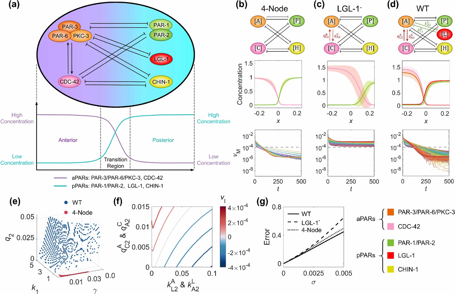
The molecular interaction network in C. *elegans* zygote and its natural advantages in terms of pattern stability, balanced network configuration, viable parameter sets, and parameter robustness.

(a) The schematic diagram of the network composed of five molecular species, each of which has a polarized spatial concentration distribution on the cell membrane shown beneath. The left nodes PAR-3/PAR-6/PKC-3 (*i.e.*, $[A]$ ) and CDC-42 (*i.e.*, $[C]$ ) exhibit high concentration in the anterior pole and low concentration in the posterior pole, schemed by the purple line beneath; the right nodes PAR-1/PAR-2 (*i.e.*, $[P]$ ), LGL-1 (*i.e.*, $[L]$ ), and CHIN-1 (*i.e.*, $[H]$ ) exhibit low concentration in the anterior pole and high concentration in the posterior pole, schemed by the cyan line beneath. Note that within the network, normal arrows and blunt arrows symbolize activation and inhibition respectively. (**b–d**) The structure of 4-Node, LGL-1^-, and WT networks (1^st row). The final spatial concentration distribution ( $t = 500$ ) averaged over all established viable parameter sets for each molecular species (*i.e.*, 62 among 262,701 sets,~0.024%, for the 4-Node network; 62 among 5,151 sets,~1.2%, for the LGL-1^- network; 602 among 262,701 sets,~0.229%, for the WT network), shown by a solid line (2^nd row). For each position, MEAN ±STD (*i.e.*, standard deviation) calculated with all viable parameter sets is shown by shadow. The pattern movement velocity ( $v_{M}$ ) over evolution time ( $t$ ) (3^rd row). For each subfigure in the 3^rd row, each line with a unique color represents the simulation of a unique viable parameter set, and $v_{M} = 10^{- 4}$ is marked by a gray dashed line. For (**a–d**), the legend for the relationship between molecular species and corresponding color is placed in the bottom right corner. (e) The viable parameter sets of WT (blue points; 602 among 262,701 sets, ~0.229%) and 4-Node networks (red points; 62 among 5,151 sets, ~1.2%). (f) The interplay between $[A]$ ~ $[C]$ mutual activation and $[A]$ ~ $[L]$ mutual inhibition on the interface velocity. The contour map of the interface velocity $v_{I}$ with different parameter combinations of $q_{C 2}^{A} & q_{A 2}^{C}$ and $k_{L 2}^{A} & k_{A 2}^{L}$ represents its moving trend. The darker the red is, the faster the interface is moving toward the posterior pole; the darker the blue is, the faster the interface is moving toward the anterior pole; the closer the color is to white, the stabler the interface is. (g) The averaged pattern error in a perturbed condition compared to the original 4-Node, LGL-1^-, and WT networks. The Gaussian noise is simultaneously exerted on all the parameters $γ$ , $α$ , $k_{1}$ , $k_{2}$ , $q_{1}$ and $q_{2}$ , where standard deviation $σ$ denotes the noise amplification. For a specific noise level, the pattern error is averaged over 1,000 independent simulations.

Figure 5—figure supplement 1

Download asset Open asset

The transformation from the simple 2-node network to the C. *elegans* 5-node network.

The reconstructed *C. elegans* 5-node network (4^th row) appears to be an integration of an antagonistic 2-node network (1^st row) doubled into an antagonistic 4-node network (2^nd row) with full connections, and then augmented by the $[A]$ ~ $[C]$ mutual activation (3^rd row, left) and $[A]$ ~ $[L]$ mutual inhibition (3^rd row, right).

Figure 5—figure supplement 2

Download asset Open asset

The *in silico* perturbation experiments on $[L]$ based on the C. *elegans* modeling framework.

(a) The experimental condition (1^st row) and final spatial concentration distribution ( $t = 500$ ) averaged over all established viable parameter sets (602 among 262,701 sets, ~0.229%) for $[A]$ and $[C]$ (2^nd row) (Hoege et al., 2010). The perturbed conditions with depletion on $[P]$ (solid line in 2^nd column), $[L]$ (solid line in 3^rd column), or both (solid line in 4^th column) are compared with the wild-type one (solid line in 1^st column and dashed line in 2^nd, 3^rd, and 4^th columns). (b) The pattern error in *C. elegans* mutant networks with depletion on $[P]$ , $[L]$ , or both (shown from left to right), compared to the pattern in *C. elegans* wild-type network. (c) The perturbed conditions (1^st row) and final spatial concentration distribution ( $t = 500$ ) averaged over all established viable parameter sets (602 among 262,701 sets,~0.229%) for $[A]$ and $[C]$ (2^nd row; Beatty et al., 2010; Beatty et al., 2013). The perturbed conditions with depletion on $[P]$ (solid line in 2^nd column), depletion on $[P]$ but overexpression of $[L]$ ( $[L_{c}]$ increased from 1 to 1.5) (solid line in 3^rd column), and depletion on both $[P]$ and $[H]$ but overexpression of $[L]$ ( $[L_{c}]$ increased from 1 to 1.5) (solid line in 4^th column) are compared with the wild-type one (solid line in 1^st column and dashed line in 2^nd, 3^rd, and 4^th columns). (d) The pattern error in *C. elegans* mutant networks with depletion on $[P]$ or both $[P]$ and $[H]$ but overexpression of $[L]$ ( $[L_{c}]$ increased from 1 to 1.5), compared to the pattern in *C. elegans* wild-type network. For (a) (c), within a network, normal arrows and blunt arrows symbolize activation and inhibition respectively. For (b) (d), the pattern error is shown by a bar chart with the average of all viable parameter sets (602 among 262,701 sets, ~0.229%), while the values from each viable parameter set are plotted with gray dots, and the ones from the same viable parameter set but in different networks are connected with gray lines.

Figure 5—figure supplement 3

Download asset Open asset

The *in silico* perturbation experiments on $[C]$ based on the C. *elegans* modeling framework.

The experimental condition (1^st row) and final spatial concentration distribution ( $t = 500$ ) averaged over all established viable parameter sets (602 among 262,701 sets,~0.229%) (2^nd row) (Gotta et al., 2001; Aceto et al., 2006). The perturbed conditions with depletion on $[C]$ (2^nd column, (b)), overexpression of $[C]$ ( $[C_{c}]$ increased from 1 to 1.5, 3^rd column, (c)), and removal of $[A]$ ~ $[C]$ mutual activation (4^th column, (d)) are compared with the wild-type one (1^st column, (a)). Note that within a network, normal arrows and blunt arrows symbolize activation and inhibition respectively.

Figure 5—figure supplement 4

Download asset Open asset

With different initial spatial concentration distributions on the cell membrane, the single modification on the C. *elegans* 5-node network causes the collapse of cell polarization pattern.

Initial distributions are shown in the 1^st column, which are the same as those shown in Figure 1—figure supplement 2d (2^nd row), Figure 1—figure supplement 2e (3^rd row), and Figure 1—figure supplement 2g (4^th row), alongside the basic network (2^nd column) and the ones with removal of single-sided self-regulation (exemplified by $[A]$ ~ $[C]$ mutual activation, 3^rd column) and single-sided additional regulation (exemplified by $[A]$ ~ $[L]$ mutual inhibition, 4^th column), and added with unequal system parameters (exemplified by unequal inhibition intensity, where $k_{L 2}^{A}$ is increased from 1 to 1.6, 5^th column; exemplified by unequal cytoplasmic concentration, where $[L_{c}]$ is increased from 1 to 1.25, 6^th column) shown on top. For each simulation, the corresponding spatial concentration distribution of $[A_{m}]$ , $[C_{m}]$ , $[P_{m}]$ , $[L_{m}]$ , and $[H_{m}]$ at are shown beneath with a color scheme listed in the bottom right corner. Note that within a network, normal arrows and blunt arrows symbolize activation and inhibition respectively. Note that within a simulation, the mathematical expressions for the initial distributions are described on the right (upper: $[A_{m}]$ and $[C_{m}]$ ; lower: $[P_{m}]$ , $[L_{m}]$ , and $[H_{m}]$ ).

Figure 5—figure supplement 5

Download asset Open asset

The 32 possible additional feedback loops between LGL-1 (*abbr*. , $[L]$ ) and PAR-3/PAR-6/PKC-3 (*abbr*., $[A]$ ) or PAR-1/PAR-2 (*abbr*., $[P]$ ).

The position of nodes on the left and right represents that the corresponding molecular species is initially set with a high concentration on the anterior and posterior cell membrane respectively. Note that within a network, normal arrows and blunt arrows symbolize activation and inhibition respectively, while dashed lines mean no regulation.

Figure 5—video 1

Download asset

Figure 6 with 1 supplement

Download asset Open asset

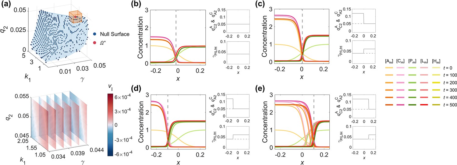
The control of the interface velocity and position by adjusting parameters in a multi-dimensional system.

(a) The parameter space (1^st row) and the linear relationship (2^nd row) between interface velocity and parameters. The discrete viable parameter space of the WT network is fitted by a blue curved surface to represent its null surface with little or no pattern interface moving (1^st row). The benchmark point $Ω^{*} (γ^{*} = 0.039, k_{1}^{*} = 1.55, q_{2}^{*} = 0.05)$ and its neighborhood are marked by an orange cube. Centering on the benchmark point $Ω^{*}$ , the relationship between the velocity interface and parameters in the region marked by the orange cube is shown by slice planes orthogonal to the $γ$ -axis at the values 0.034, 0.036, 0.038, 0.04, 0.042, and 0.044 (2^nd row). The darker the red is, the faster the interface is moving toward the posterior pole; the darker the blue is, the faster the interface is moving toward the anterior pole; the closer the color is to white, the stabler the interface is. (**b–e**) As in Figure 4, the control of the zero-velocity interface position of the polarity pattern by spatially inhomogeneous parameters corresponding to opposite interface velocities on two sides of the interface can be applied to the *C. elegans* 5-node network. (b) Using $Ω^{*}$ as a representative, spatially homogeneous parameters (2^nd column) generate a stable polarity pattern (1^st column). (c) On top of (b), a stable polarity pattern (1^st column) with its interface around $x = 0$ can be obtained by increasing $q_{C 2}^{A}$ & $q_{A 2}^{C}$ to 0.12 at $x < 0$ and increasing $γ_{P}, γ_{L}, a n d γ_{H}$ to 0.06 at $x > 0$ (2^nd column). (d) As in (c) but changing the step position to $x = - 0.1$ (2^nd column), the interface stabilizes around $x = - 0.1$ (1^st column). (e) As in (c), but changing the step position to $x = 0.1$ (2^nd column), the interface stabilizes around $x = 0.1$ (1^st column). For each parameter set, the corresponding spatial concentration distribution of $[A_{m}]$ , $[C_{m}]$ , $[P_{m}]$ , $[L_{m}]$ , and $[H_{m}]$ at $t = 0, 100, 200, 300, 400, a n d 500$ are shown beneath with a color scheme listed on the right. Note that all the interface positions in (**b–e**) (1^st column) are marked by gray dashed lines. Note that all the spatially homogeneous parameter distributions in (b) (2^nd column) are marked by gray dashed lines in (**c–e**) (2^nd column).

Figure 6—video 1

Download asset

Appendix 2—figure 1

Download asset Open asset

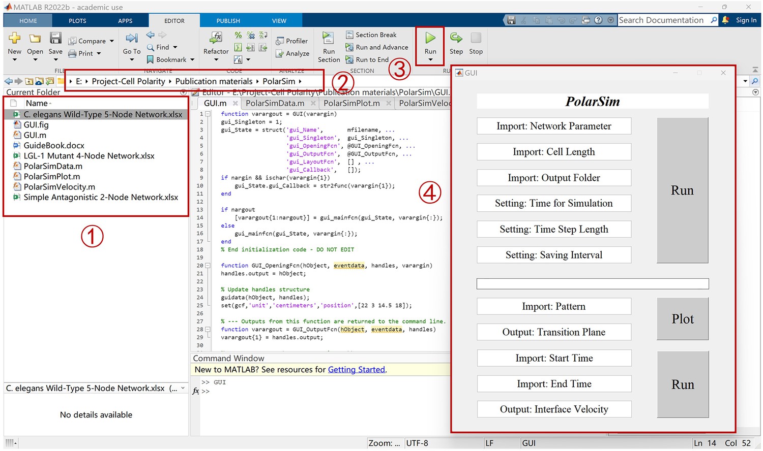
The instructions to open the *PolarSim* GUI.

① The files in the folder ‘PolarSim’. ② Open *Matlab* under the path of the folder ‘PolarSim’ and double-click to open ‘GUI.m’. ③ Click ‘Run’ to open the *PolarSim* GUI shown by ④.

Appendix 2—figure 2

Download asset Open asset

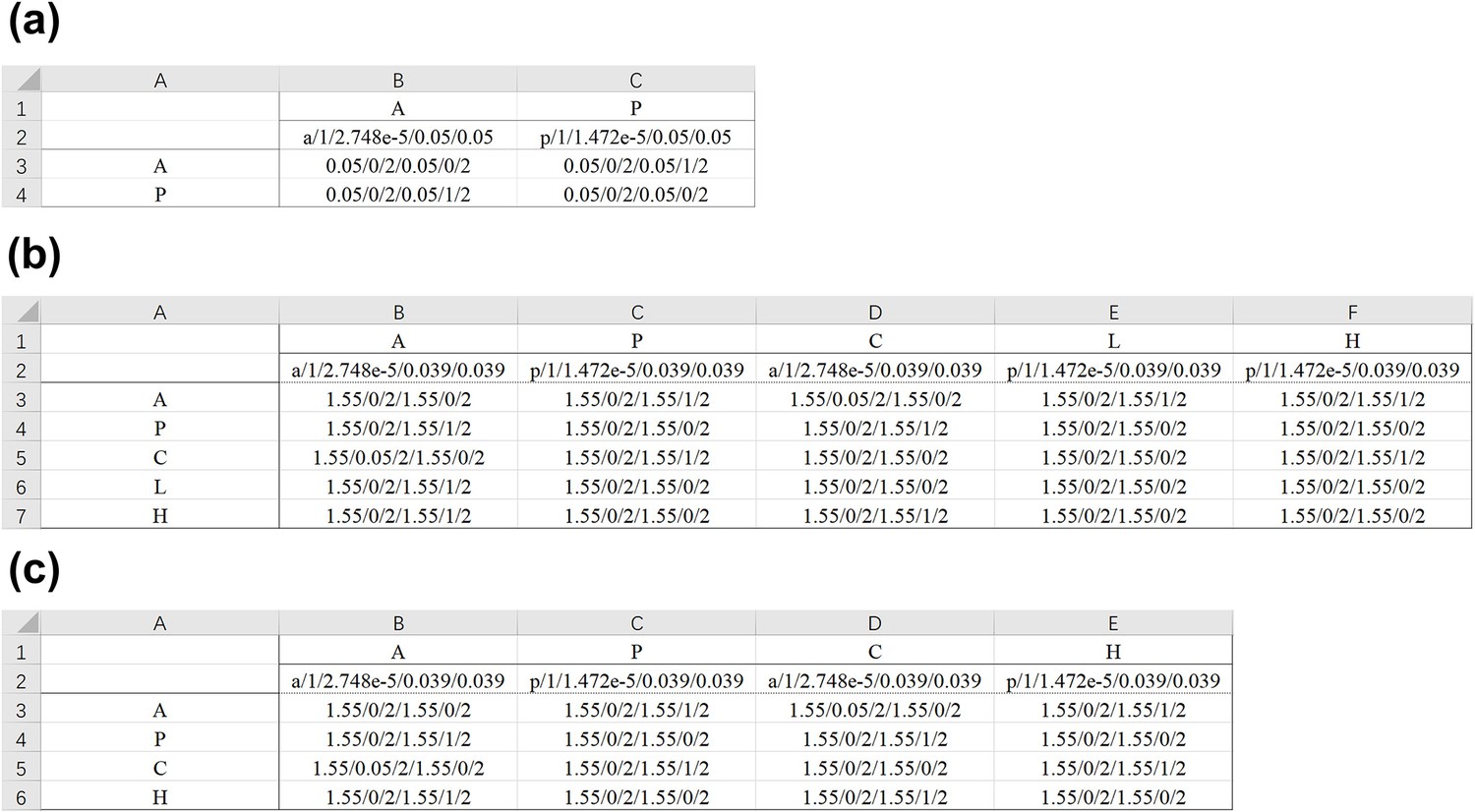
The examples of network parameters.

(a) ‘Simple Antagonistic 2-Node Network.xlsx lists the parameters’ in Figure 1a. (b) ‘C. elegans Wild-Type 5-Node Network.xlsx’ lists the parameters for the benchmark point $Ω^{*} (γ^{*} = 0.039, k_{1}^{*} = 1.55, q_{2}^{*} = 0.05)$ in Figure 6b. (c) ‘LGL-1 Mutant 4-Node Network.xlsx’ lists the parameters as in (b) but with the Node $[L]$ knocked out.

Appendix 2—figure 3

Download asset Open asset

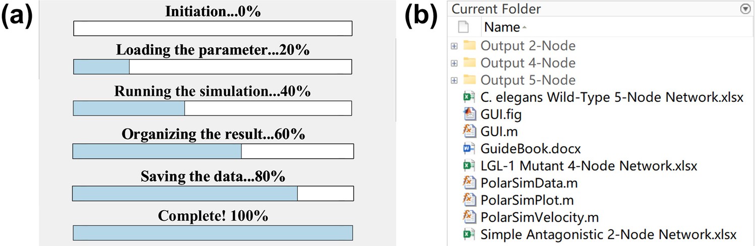
The progress bar, files, and subfolders of *PolarSim*.

(a) The progress bar showing the running progress. (b) All files and output subfolders in the folder ‘PolarSim’.

Appendix 2—figure 4

Download asset Open asset

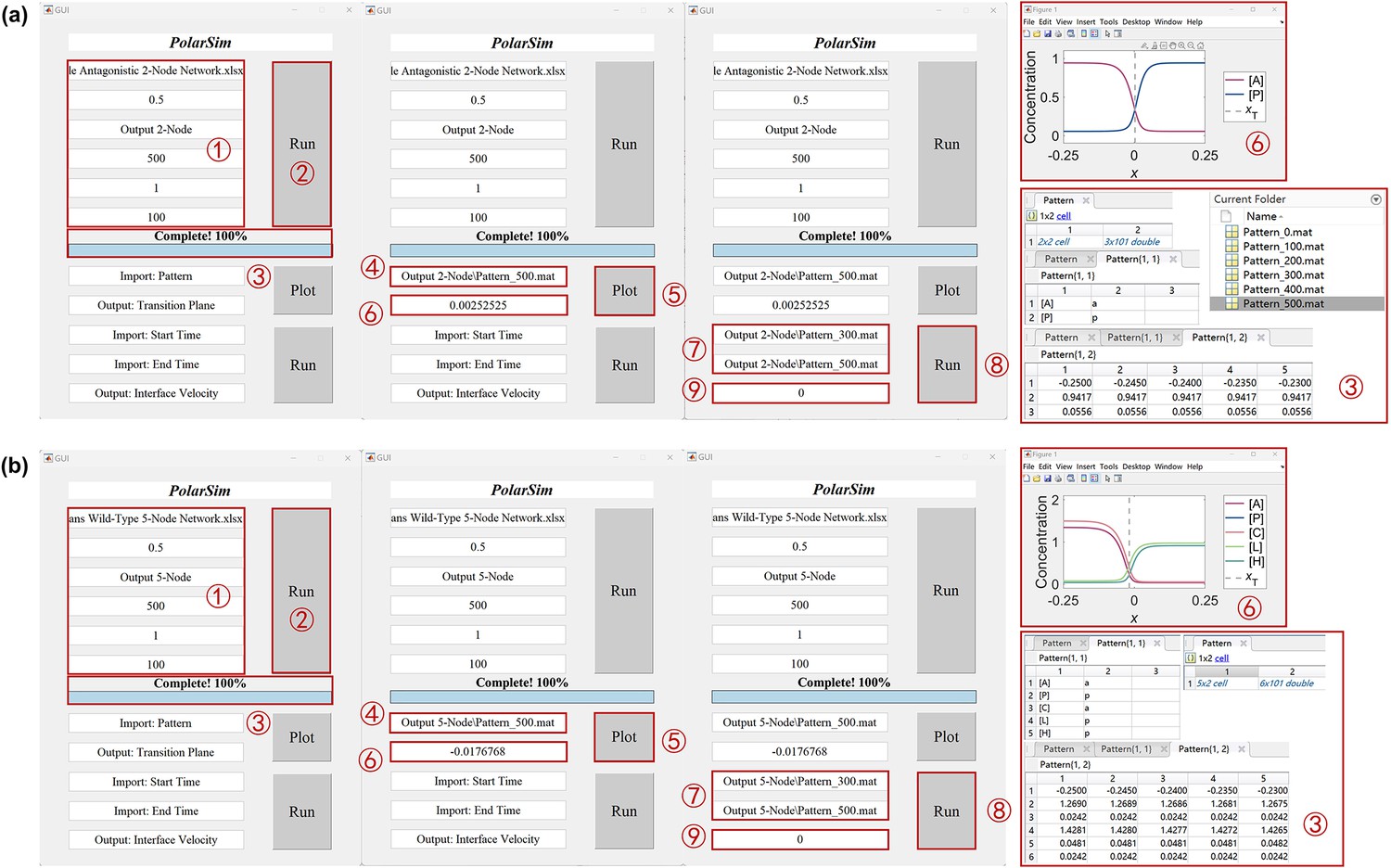
The results of Example 1 (‘Simple Antagonistic 2-Node Network.xlsx’) and Example 2 (‘C. elegans Wild-Type 5-Node Network.xlsx’) of *PolarSim*.

(a) The flow chart for computing Example 1: ① input parameters; ② click ‘Run’; ③ the simulation is completed with a progress bar shown and files saved in the folder ‘Output 2-Node’; the file ‘Pattern_500.mat’ is used to show the data format on the right, where the first part stores the molecular species or nodes’ names and locations while the second part stores their spatial concentration distributions on the cell membrane; ④ input the pathway of the outputted pattern file; ⑤ click ‘Plot’; ⑥ the simulation is completed with a figure shown and the position of the transition plane given in the box ‘Output: Transition Plane’; ⑦ input the pathway of the two outputted files ‘Pattern_*.mat’ at different time points into ‘Import: Start Time’ and ‘Import: End Time’, where ‘*’ denotes the start time and end time respectively; ⑧ click ‘Run’; ⑨ the simulation is completed with the interface velocity given in the box ‘Output: Interface Velocity’. (b) The same as a but for the ‘C. elegans Wild-Type 5-Node Network.xlsx’.

Appendix 2—figure 5

Download asset Open asset

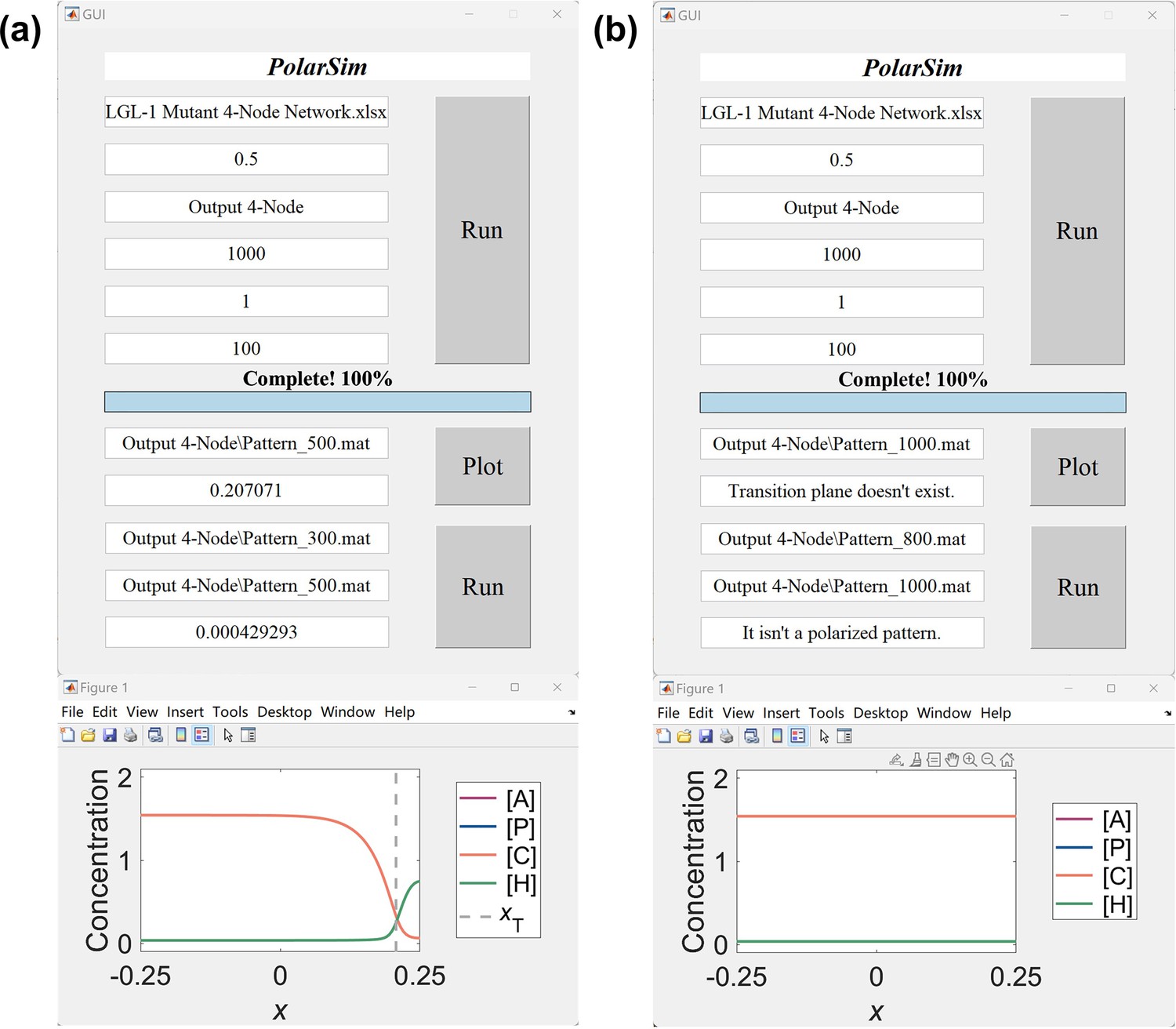
The results of Example 3 (‘LGL-1 Mutant 4-Node Network.xlsx’) of *PolarSim*.

(a) The transition plane is shown at $t = 500$ , with the value $x_{T} = 0.207071$ . The interface velocity is calculated between $t = 300$ and $t = 500$ , with the value $v_{I} = 0.000429293$ representing an unstable pattern (top). The figure is plotted at $t = 500$ (bottom). (b) The transition plane and the figure are shown at $t = 1000$ and the interface velocity is calculated between $t = 800$ and $t = 1000$ . The pattern collapses to a homogeneous state with $[A]$ and $[C]$ invading the posterior domain at $t = 1000$ , and thereby the transition plane doesn’t exist and the interface can’t be calculated.

Appendix 2—figure 6

Download asset Open asset

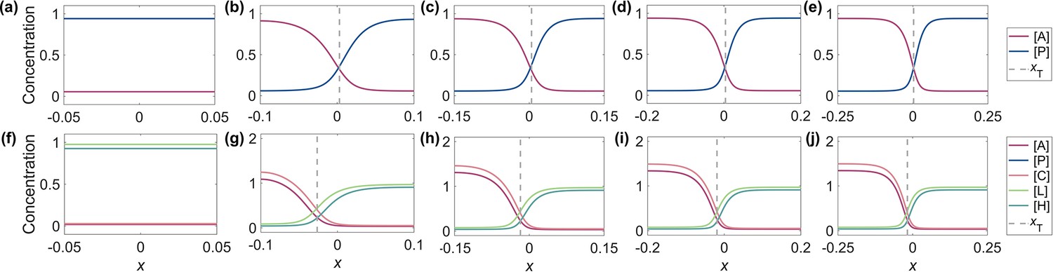
The effects of cell size (length) on the cell polarization pattern.

(**a–e**) The pattern of ‘Simple Antagonistic 2-Node Network.xlsx’ at $t = 500$ . From left to right, the cell lengths are 0.1, 0.2, 0.3, 0.4 and 0.5, respectively. (**f–j**) The same as (**a–e**) but for the ‘C. elegans Wild-Type 5-Node Network.xlsx’.

Tables

Appendix 1—table 1

The parameter description of the reaction-diffusion model for simulating a cell polarization network.

Parameter	Biological implication	Defaulted nondimensionalvalue in simulation
$x$	Position along the anterior-posterior axis	[–0.25,0.25] in steps 0.005
$t$	Time	[0,500] in steps 1 (corresponding to 2 sec per step) ( Blanchoud et al., 2015; Seirin-Lee et al., 2020b)
$[X]$	Molecular species	/
$[X_{m}]$	Spatial concentration distribution on the cell membrane	/
$[X_{c}]$	Spatial concentration distribution in the cell cytosol	1
$D_{m}^{X}$	Diffusion coefficient across the cell membrane	2.748×10^–5 for anteriorly-located molecular species and 1.472×10^–5 for posteriorly-located molecular species (Goehring et al., 2011a; Goehring et al., 2011b; Geßele et al., 2020; Seirin-Lee et al., 2020b)
$γ_{X}$	Basal on-rate (cell membrane association)	[0,0.05] in steps 0.001
$α_{X}$	Basal off-rate (cell membrane dissociation)	[0,0.05] in steps 0.001
$q_{Y 1}^{X}$	Responsive concentration in the activation pathway from $[Y]$ to $[X]$	[0,5] in steps 0.05
$k_{Y 1}^{X}$	Responsive concentration in the inhibition pathway from $[Y]$ to $[X]$	[0,5] in steps 0.05
$q_{Y 2}^{X}$	Activation intensity from $[Y]$ to $[X]$	[0,0.05] in steps 0.001
$k_{Y 2}^{X}$	Inhibition intensity from $[Y]$ to $[X]$	1
$Ω$	A three-dimensional (3D) grid representing nondimensionalized parameter set	$(γ, k_{1}, q_{2})$
$n$	Hill coefficient	2 (Seirin-Lee and Shibata, 2015; Seirin-Lee, 2021)
$L$	Cell/embryo length	0.5
$v_{M}$	Pattern movement velocity	/
$x_{T}$	Pattern transition plane or interface	/
$v_{I}$	Interface velocity	/
$N$	Number of molecular species types	/
$M$	Number of viable parameter sets	/
$Q$	Number of independent simulations	/

Appendix 1—table 2

Viable parameter set searched by Monte Carlo method for the simple 2-node network.

For the 10 parameters in the simple 2-node network, the corresponding scanned ranges are $γ \in [0, 0.05], α \in [0, 0.05], k_{1} \in [0.05, 5], k_{2} \in [0.05, 5]$ , and . Among 100,000 independent simulations, only 20 viable parameter sets pass the computational pipeline. One representative viable parameter set used to reproduce the conclusions in Figure 1; Figure 1—figure supplement 5 -1^st row is listed below.

Parameter	NondimensionalValue in Simulation	Parameter	NondimensionalValue in Simulation
$[A_{c}]$	1.5361	$[P_{c}]$	0.6662
$γ_{A}$	0.0251	$α_{A}$	0.0437
$γ_{P}$	0.0312	$α_{P}$	0.0245
$k_{P 1}^{A}$	0.1995	$k_{P 2}^{A}$	3.8471
$k_{A 1}^{P}$	1.3638	$k_{A 2}^{P}$	2.2571

Appendix 1—table 3

Viable parameter set searched by Monte Carlo method for the C. elegans 5-node network.

For the 39 parameters in the C. elegans 5-node network, the corresponding scanned ranges are $γ \in [0, 0.05], α \in [0, 0.05], k_{1} \in [0.05, 5], k_{2} \in [0.05, 5], q_{1} \in [0.05, 5], q_{2} \in [0, 0.05]$ , and $[X_{c}] \in [0.05, 5]$ . Among 100,000 independent simulations, only 6 viable parameter sets pass the computational pipeline. One representative viable parameter set used to reproduce the conclusions in Figure 1; Figure 1—figure supplement 5 -2^nd row is listed below.

Parameter	NondimensionalValue in Simulation	Parameter	NondimensionalValue in Simulation
$[A_{c}]$	2.4420	$[P_{c}]$	3.6739
$[C_{c}]$	1.8330	$[L_{c}]$	2.3793
$[H_{c}]$	3.4683
$γ_{A}$	0.0448	$α_{A}$	0.0310
$γ_{P}$	0.0164	$α_{P}$	0.0334
$γ_{C}$	0.0158	$α_{C}$	0.0071
$γ_{L}$	0.0146	$α_{L}$	0.0221
$γ_{H}$	0.0197	$α_{H}$	0.0410
$q_{A 1}^{C}$	4.1521	$q_{A 2}^{C}$	0.0495
$q_{C 1}^{A}$	1.3029	$q_{C 2}^{A}$	0.0201
$k_{P 1}^{A}$	3.7955	$k_{P 2}^{A}$	0.2009
$k_{L 1}^{A}$	2.3597	$k_{L 2}^{A}$	3.7357
$k_{H 1}^{A}$	1.9557	$k_{H 2}^{A}$	2.2441
$k_{A 1}^{P}$	3.7180	$k_{A 2}^{P}$	3.7342
$k_{C 1}^{P}$	4.5544	$k_{C 2}^{P}$	1.5792
$k_{P 1}^{C}$	0.5495	$k_{P 2}^{C}$	2.8838
$k_{H 1}^{C}$	2.6518	$k_{H 2}^{C}$	1.2697
$k_{A 1}^{L}$	2.4436	$k_{A 2}^{L}$	4.8334
$k_{A 1}^{H}$	4.4505	$k_{A 2}^{H}$	0.3688
$k_{C 1}^{H}$	3.3712	$k_{C 2}^{H}$	2.0272

Appendix 2—table 1

The instructions for the format of Network Parameter in an Excel table.

In the 1^st row and 1^st column, ‘Node N’ represents the name of the node. The 2^nd row explains the characteristic parameters of each node (i.e., location, cytoplasmic concentration, basal on-rate, and basal off-rate as listed from left to right). The interaction parameters start from the 3^rd row and 2^nd column, where the i^th row and j^th column describe the activation/inhibition effect from Node j to Node i. Note that $q_{Y 2}^{X}$ and $k_{Y 2}^{X}$ should be set to 0 when no activation or inhibition is exerted on X from Y respectively. ‘Location’ should be assigned with the string ‘a’ or ‘p’ while the description of the other parameters is detailed in Appendix 1—table 1.

	Node A	Node B	…	Node N
	Location (a or p)/ $[A_{c}]$ / $γ_{A}$ / $α_{A}$	Location (a or p)/ $[B_{c}]$ / $γ_{B}$ / $α_{B}$	…	Location (a or p)/ $[N_{c}]$ / $γ_{N}$ / $α_{N}$
Node A	$q_{A 1}^{A}$ / $q_{A 2}^{A}$ / $n_{A q}^{A}$ / $k_{A 1}^{A}$ / $k_{A 2}^{A}$ / $n_{A k}^{A}$	$q_{B 1}^{A}$ / $q_{B 2}^{A}$ / $n_{B q}^{A}$ / $k_{B 1}^{A}$ / $k_{B 2}^{A}$ / $n_{B k}^{A}$	…	$q_{N 1}^{A}$ / $q_{N 2}^{A}$ / $n_{N q}^{A}$ / $k_{N 1}^{A}$ / $k_{N 2}^{A}$ / $n_{N k}^{A}$
Node B	$q_{A 1}^{B}$ / $q_{A 2}^{B}$ / $n_{A q}^{B}$ / $k_{A 1}^{B}$ / $k_{A 2}^{B}$ / $n_{A k}^{B}$	$q_{B 1}^{B}$ / $q_{B 2}^{B}$ / $n_{B q}^{B}$ / $k_{B 1}^{B}$ / $k_{B 2}^{B}$ / $n_{B k}^{B}$	…	$q_{N 1}^{B}$ / $q_{N 2}^{B}$ / $n_{N q}^{B}$ / $k_{N 1}^{B}$ / $k_{N 2}^{B}$ / $n_{N k}^{B}$
…	…	…	…	…
Node N	$q_{A 1}^{N}$ / $q_{A 2}^{N}$ / $n_{A q}^{N}$ / $k_{A 1}^{N}$ / $k_{A 2}^{N}$ / $n_{A k}^{N}$	$q_{B 1}^{N}$ / $q_{B 2}^{N}$ / $n_{B q}^{N}$ / $k_{B 1}^{N}$ / $k_{B 2}^{N}$ / $n_{B k}^{N}$	…	$q_{N 1}^{N}$ / $q_{N 2}^{N}$ / $n_{N q}^{N}$ / $k_{N 1}^{N}$ / $k_{N 2}^{N}$ / $n_{N k}^{N}$

Additional files

Supplementary file 1 The literature summary on the cell polarization network in the C. elegans zygote.: https://cdn.elifesciences.org/articles/96421/elife-96421-supp1-v1.xlsx
Download elife-96421-supp1-v1.xlsx
MDAR checklist: https://cdn.elifesciences.org/articles/96421/elife-96421-mdarchecklist1-v1.docx
Download elife-96421-mdarchecklist1-v1.docx
Source code 1 The scripts and guidebook of the software PolarSim GUI.: https://cdn.elifesciences.org/articles/96421/elife-96421-code1-v1.zip
Download elife-96421-code1-v1.zip

Download links

A two-part list of links to download the article, or parts of the article, in various formats.

Downloads (link to download the article as PDF)

Open citations (links to open the citations from this article in various online reference manager services)

Mendeley

Cite this article (links to download the citations from this article in formats compatible with various reference manager tools)

Yixuan Chen
Guoye Guan
Lei-Han Tang
Chao Tang

(2025)

Balancing reaction-diffusion network for cell polarization pattern with stability and asymmetry

eLife 13:RP96421.

https://doi.org/10.7554/eLife.96421.3

Share this article

Cite this article

The single modification on the antagonistic 2-node network causes the collapse of cell polarization pattern.

The initial state at t=0 (shown on the left) and stable state at t=500 (shown in the middle) of the cell polarization pattern generated by the simple 2-node network and C. elegans 5-node network (shown on the right).

The antagonistic 2-node network initiated with different initial spatial concentration distributions on the cell membrane.

The antagonistic 2-node network added with four subtypes of single-sided additional regulation (corresponding to Figure 1c) causes the collapse of cell polarization pattern.

With different initial spatial concentration distributions on the cell membrane, the single modification on the antagonistic 2-node network causes the collapse of cell polarization pattern.

The spatial concentration distribution of each molecular species on the cell membrane over time generated by the antagonistic 2-node network and the ones with a single modification added, corresponding to Figure 1.

The combination of two opposite modifications recovers the cell polarization pattern stability.

The spatial concentration distribution of each molecular species on the cell membrane over time generated by the antagonistic 2-node network and the ones with a single modification or two combinatorial modifications added, corresponding to Figure 2.

The balance between system parameters is needed for maintaining pattern stability.

Adopting parameter sets corresponding to opposite interface velocities on two sides of the interface, the zero-velocity interface position of the polarity pattern is shiftable and regulatable.

The spatial concentration distribution of each molecular species on the cell membrane over time generated by the antagonistic 2-node network with spatially inhomogeneous parameters, corresponding to Figure 4.

The molecular interaction network in C. elegans zygote and its natural advantages in terms of pattern stability, balanced network configuration, viable parameter sets, and parameter robustness.

The transformation from the simple 2-node network to the C. elegans 5-node network.

The in silico perturbation experiments on [L] based on the C. elegans modeling framework.

The in silico perturbation experiments on [C] based on the C. elegans modeling framework.

With different initial spatial concentration distributions on the cell membrane, the single modification on the C. elegans 5-node network causes the collapse of cell polarization pattern.

The 32 possible additional feedback loops between LGL-1 (abbr. , [L]) and PAR-3/PAR-6/PKC-3 (abbr., [A]) or PAR-1/PAR-2 (abbr., [P]).

The spatial concentration distribution of each molecular species on the cell membrane over time generated by the 4-Node, LGL-1-, and WT networks, corresponding to Figure 5b–d.

The control of the interface velocity and position by adjusting parameters in a multi-dimensional system.

The spatial concentration distribution of each molecular species on the cell membrane over time generated by the C. elegans 5-node network with spatially inhomogeneous parameters, corresponding to Figure 6b–e.

The instructions to open the PolarSim GUI.

The examples of network parameters.

The progress bar, files, and subfolders of PolarSim.

The results of Example 1 (‘Simple Antagonistic 2-Node Network.xlsx’) and Example 2 (‘C. elegans Wild-Type 5-Node Network.xlsx’) of PolarSim.

The results of Example 3 (‘LGL-1 Mutant 4-Node Network.xlsx’) of PolarSim.

The effects of cell size (length) on the cell polarization pattern.

The parameter description of the reaction-diffusion model for simulating a cell polarization network.

Viable parameter set searched by Monte Carlo method for the simple 2-node network.

Viable parameter set searched by Monte Carlo method for the C. elegans 5-node network.

The instructions for the format of Network Parameter in an Excel table.

Supplementary file 1

MDAR checklist

Source code 1

Downloads (link to download the article as PDF)

Open citations (links to open the citations from this article in various online reference manager services)

Cite this article (links to download the citations from this article in formats compatible with various reference manager tools)

The initial state at $t = 0$ (shown on the left) and stable state at $t = 500$ (shown in the middle) of the cell polarization pattern generated by the simple 2-node network and C. elegans 5-node network (shown on the right).

The in silico perturbation experiments on $[L]$ based on the C. elegans modeling framework.

The in silico perturbation experiments on $[C]$ based on the C. elegans modeling framework.

The 32 possible additional feedback loops between LGL-1 (abbr. , $[L]$ ) and PAR-3/PAR-6/PKC-3 (abbr., $[A]$ ) or PAR-1/PAR-2 (abbr., $[P]$ ).

The spatial concentration distribution of each molecular species on the cell membrane over time generated by the 4-Node, LGL-1^-, and WT networks, corresponding to Figure 5b–d.