Neural coding of multiple motion speeds in visual cortical area MT

Reviewer #1 (Public review):

Summary:

Most studies in sensory neuroscience investigate how individual sensory stimuli are represented in the brain (e.g., the motion or color of a single object). This study starts tackling the more difficult question of how the brain represents multiple stimuli simultaneously and how these representations help to segregate objects from cluttered scenes with overlapping objects.

Strengths

The authors first document the ability of humans to segregate two motion patterns based on differences in speed. Then they show that a monkey's performance is largely similar; thus establishing the monkey as a good model to study the underlying neural representations.

Careful quantification of the neural responses in the middle temporal area during the simultaneous presentation of fast and slow speeds leads to the surprising finding that, at low average speeds, many neurons respond as if the slowest speed is not present, while they show averaged responses at high speeds. This unexpected complexity of the integration of multiple stimuli is key to the model developed in this paper.

One experiment in which attention is drawn away from the receptive field supports the claim that this is not due to the involuntary capture of attention by fast speeds.

A classifier using the neuronal response and trained to distinguish single speed from bi-speed stimuli shows a similar overall performance and dependence on the mean speed as the monkey. This supports the claim that these neurons may indeed underlie the animal's decision process.

The authors expand the well-established divisive normalization model to capture the responses to bi-speed stimuli. The incremental modeling (eq 9 and 10) clarifies which aspects of the tuning curves are captured by the parameters.

Reviewer #3 (Public review):

Summary:

This study concerns how macaque visual cortical area MT represents stimuli composed of more than one speed of motion.

Strengths:

The study is valuable because little is known about how the visual pathway segments and preserves information about multiple stimuli. The study presents compelling evidence that (on average) MT neurons shift from faster-speed-takes-all at low speeds to representing the average of the two speeds at higher speeds. An additional strength of the study is the inclusion of perceptual reports from both humans and one monkey participant performing a task in which they judged whether the stimuli involved one vs two different speeds. Ultimately, this study raises intriguing questions about how exactly the response patterns in visual cortical area MT might preserve information about each speed, since such information is potentially lost in an average response as described here.

Author response:

The following is the authors’ response to the original reviews

Public Reviews:

Reviewer #1 (Public Review):

Summary:

Most studies in sensory neuroscience investigate how individual sensory stimuli are represented in the brain (e.g., the motion or color of a single object). This study starts tackling the more difficult question of how the brain represents multiple stimuli simultaneously and how these representations help to segregate objects from cluttered scenes with overlapping objects.

Strengths

The authors first document the ability of humans to segregate two motion patterns based on differences in speed. Then they show that a monkey's performance is largely similar; thus establishing the monkey as a good model to study the underlying neural representations.

Careful quantification of the neural responses in the middle temporal area during the simultaneous presentation of fast and slow speeds leads to the surprising finding that, at low average speeds, many neurons respond as if the slowest speed is not present, while they show averaged responses at high speeds. This unexpected complexity of the integration of multiple stimuli is key to the model developed in this paper.

One experiment in which attention is drawn away from the receptive field supports the claim that this is not due to the involuntary capture of attention by fast speeds.

A classifier using the neuronal response and trained to distinguish single-speed from bi-speed stimuli shows a similar overall performance and dependence on the mean speed as the monkey. This supports the claim that these neurons may indeed underlie the animal's decision process.

The authors expand the well-established divisive normalization model to capture the responses to bi-speed stimuli. The incremental modeling (eq 9 and 10) clarifies which aspects of the tuning curves are captured by the parameters.

We thank the Reviewer for the thorough summary of the findings and supportive comments.

Weaknesses

While the comparison of the overall pattern of behavioral performance between monkeys and humans is important, some of the detailed comparisons are not well supported by the data. For instance, whether the monkey used the apparent coherence simply wasn't tested and a difference between 4 human subjects and a single monkey subject cannot be tested statistically in a meaningful manner. I recommend removing these observations from the manuscript and leaving it at "The difference between the monkey and human results may be due to species differences or individual variability" (and potentially add that there are differences in the task as well; the monkey received feedback on the correctness of their choice, while the humans did not.)

Thanks for the suggestion. We agree and have modified the text accordingly. We now state on page 8, lines 189-191, "The difference between the monkey and human results may be due to species differences or individual variability. The differences in behavioral tasks may also play a role – the monkey received feedback on the correctness of the choice, whereas human subjects did not."

A control experiment aims to show that the "fastest speed takes all" behavior is general by presenting two stimuli that move at fast/slow speeds in orthogonal directions. The claim that these responses also show the "fastest speed takes all" is not well supported by the data. In fact, for directions in which the slow speed leads to the largest response on its own, the population response to the bi-speed stimulus is the average of the response to the components (This is fine. One model can explain all direction tuning curve, which also explain averaging at the slower speed stronger directions). Only for the directions where the fast speed stimulus is the preferred direction is there a bias towards the faster speed (Figure 7A). The quantification of this effect in Figure 7B seems to suggest otherwise, but I suspect that this is driven by the larger amplitude of Rf in Figure 8, and the constraint that ws and wf are constant across directions. The interpretation of this experiment needs to be reconsidered.

The Reviewer raised a good question. Our model with fixed weights for faster and slower components across stimulus directions provided a parsimonious explanation for the whole tuning curve, regardless of whether the faster component elicited a stronger response than the slower component. Because the model can be well constrained by the measured direction-tuning curves, we did not restrain 𝑤 and 𝑤 to sum to one, which is more general. The linear weighted summation (LWS) model fits the neuronal responses to the bi-speed stimuli very well, accounting for an average of 91.8% (std = 7.2%) of the response variance across neurons. As suggested by the Reviewer, we now use the normalization model to fit the data with fixed weights across all motion directions. The normalization model also provides a good fit, accounting for an average of 90.5% (std = 7.1%) of the response variance across neurons.

Note that in the new Figure 8A, at the left side of the tuning curve (i.e., at negative vector average (VA) directions), where the slower component moving in a more preferred direction of the neurons than the faster component, the bi-speed response (red curve) is slightly lower than the average of the component response (gray curve), indicating a bias toward the weaker faster component. Therefore, the faster speed bias does not occur only when the faster component moves in the more preferred direction. This can also be seen in the direction-tuning curves of an example neuron that we added to the figure (new Fig. 8B). The peak responses to the slower and faster component were about the same, but the neuron still showed a faster-speed bias. At negative VA directions, the red curve is lower than the response average (gray curve) and is biased toward the weaker (faster) component.

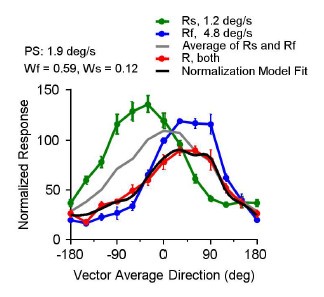
The faster-speed bias also occurs when the peak response to the slower component is stronger than the faster component. As a demonstration, Author response image 1 1 shows an example MT neuron that has a slow preferred speed (PS = 1.9 deg/s) and was stimulated by two speeds of 1.2 and 4.8 deg/s. The peak response to the faster component (blue) was weaker than that to the slower component (green). However, this neuron showed a strong bias toward the faster component. A normalization model fit with fixed weights for the faster and slower components (black curve) described the neuronal response to both speeds (red) well. This neuron was not included in the neuron population shown in Figure 8 because it was not tested with stimulus speeds of 2.5 and 10 deg/s.

Author response image 1.

An example MT neuron was tested with stimulus speeds of 1.2 and 4.8 deg/s. The preferred speed of this neuron was 1.9 deg/s. Fixed weights of 0.59 for the faster component and 0.12 for the slower component described the responses to the bispeed stimuli well using a normalization model. The neuron showed a faster-speed bias although its peak response to the slower component was higher than that of the faster component.

We modified the text to clarify these points:

Page 19, lines 405 – 410, “The bi-speed response was biased toward the faster component regardless of whether the response to the faster component was stronger (in positive VA directions) or weaker (in negative VA directions) than that to slower component (Fig. 8A). The result from an example neuron further demonstrated that, even when the peak firing rates of the faster and slower component responses were similar, the response elicited by the bi-speed stimuli was still biased toward the faster component (Fig. 8B). ”

Page 19, lines 421 – 427, “Because the model can be well constrained by the measured direction-tuning curves, it is not necessary to require 𝑤 and 𝑤 to sum to one, which is more general. An implicit assumption of the model is that, at a given pair of stimulus speeds, the response weights for the slower and faster components are fixed across motion directions. The model fitted MT responses very well, accounting for an average of 91.8% of the response variance (std = 7.2%, N = 21) (see Methods). The success of the model supports the assumption that the response weights are fixed across motion directions.”

Reviewer #2 (Public Review):

Summary:

This is a paper about the segmentation of visual stimuli based on speed cues. The experimental stimuli are random dot fields in which each dot moves at one of two velocities. By varying the difference between the two speeds, as well as the mean of the two speeds, the authors estimate the capacity of observers (human and non-human primates) to segment overlapping motion stimuli. Consistent with previous work, perceptual segmentation ability depends on the mean of the two speeds. Recordings from area MT in monkeys show that the neuronal population to compound stimuli often shows a bias towards the faster-speed stimuli. This bias can be accounted for with a computational model that modulates single-neuron firing rates by the speed preferences of the population. The authors also test the capacity of a linear classifier to produce the psychophysical results from the MT data.

Strengths:

Overall, this is a thorough treatment of the question of visual segmentation with speed cues. Previous work has mostly focused on other kinds of cues (direction, disparity, color), so the neurophysiological results are novel. The connection between MT activity and perceptual segmentation is potentially interesting, particularly as it relates to existing hypotheses about population coding.

We thank the Reviewer for the summary and comments.

Weaknesses:

Page 10: The relationship between (R-Rs) and (Rf-Rs) is described as "remarkably linear". I don't actually find this surprising, as the same term (Rs) appears on both the x- and y-axes. The R^2 values are a bit misleading for this reason.

The Reviewer is correct that subtracting a common term Rs from R and Rf would introduce correlation between (R-Rs) and (Rf-Rs). To address this concern, we conducted an additional analysis. We showed that, at most speed pairs, the R^2 values between (R-Rs) and (Rf-Rs) based on the data are significantly higher than the R^2 values between (R’-Rs) and (RfRs), in which R’ was a random combination of Rs and Rf. Since the same Rs was commonly subtracted in calculating R^2 (data) and R^2 (simulation), the difference between R^2 (data) and R^2 (simulation) suggests that the response pattern of R contributes to the additional correlation.

We now acknowledge this confounding factor and describe the new analysis results on page 14, lines 309 – 326. Please also see the response to Reviewer 3 about a similar concern.

Figure 9: I'm confused about the linear classifier section of the paper. The idea makes sense - the goal is to relate the neuronal recordings to the psychophysical data. However the results generally provide a poor quantitative match to the psychophysical data. There is mention of a "different paper" (page 26) involving a separate decoding study, as well as a preprint by Huang et al. (2023) that has better decoding results. But the Huang et al. preprint appears to be identical to the current manuscript, in that neither has a Figure 12, 13, or 14. The text also says (page 26) that the current paper is not really a decoding study, but the linear classifier (Figure 9F) is a decoder, as noted on page 10. It sounds like something got mixed up in the production of two or more papers from the same dataset.

We apologize for the confusion regarding the reference of Huang et al. (2023, bioRxiv). We referred to an earlier version of this bioRxiv manuscript (version 1), which included decoding analysis. In the bibliography, we provided two URLs for this pre-print. While the second link was correct, the first URL automatically links to the latest version (version 2), which did not have the abovementioned decoding analysis.

The analysis in Figure 9 is to apply a classifier to discriminate two-speed from singlespeed stimuli, which is a decoding analysis as the Reviewer pointed out. We revised the result section about the classifier to make it clear what the classifier can and cannot explain (pages 2223, lines 516-534). We also included a sentence at the end of this section that leads to additional decoding analysis to extract motion speed(s) from MT population responses (page 23, lines 541543), “To directly evaluate whether the population neural responses elicited by the bi-speed stimulus carry information about two speeds, it is important to conduct a decoding analysis to extract speed(s) from MT population responses.”

In any case, I think that some kind of decoding analysis would really strengthen the current paper by linking the physiology to the psychophysics, but given the limitations of the linear classifier, a more sophisticated approach might be necessary -- see for example Zemel, Dayan, and Pouget, 1998. The authors might also want to check out closely related work by Treue et al. (Nature Neuroscience 2000) and Watamaniuk and Duchon (1992).

We thank the Reviewer for the suggestion and agree that it is useful to incorporate additional decoding analysis that can better link physiology results to psychophysics. The decoding analysis we conducted was motivated by the framework proposed by Zemel, Dayan, and Pouget (1998), and also similar to the idea briefly mentioned in the Discussion of Treue et al. (2000). We have added the decoding analysis to this paper on pages 25-32.

What do we learn from the normalization model? Its formulation is mostly a restatement of the results - that the faster and slower speeds differentially affect the combined response. This hypothesis is stated quantitatively in equation 8, which seems to provide a perfectly adequate account of the data. The normalization model in equation 10 is effectively the same hypothesis, with the mean population response interposed - it's not clear how much the actual tuning curve in Figure 10A even matters, since the main effect of the model is to flatten it out by averaging the functions in Figure 10B. Although the fit to the data is reasonable, the model uses 4 parameters to fit 5 data points and is likely underconstrained; the parameters other than alpha should at least be reported, as it would seem that sigma is actually the most important one. And I think it would help to examine how robust the statistical results are to different assumptions about the normalization pool.

In the linear weighted summation model (LWS) model (Eq. 8), the weights Ws and Wf are free parameters. We think the value of the normalization model (Eq. 9) is that it provides an explanation of what determines the response weights. We agree with the Reviewer that using the normalization model (Eq. 9) with 4 parameters to fit 5 data points of the tuning curves to bispeed stimuli of individual neurons is under-constrained. We, therefore, removed the section using the normalization model to fit overlapping stimuli moving in the same direction at different speeds.

A better way to constrain the normalization model is to use the full direction-tuning curves of MT neurons in response to two stimulus components moving in different directions at different speeds, as shown in Figure 8. We now use the normalization model (Eq. 9) to fit this data set (also suggested by Reviewer 1), in addition to the LWS model. We now report the median values of the model parameters of the normalization model, including the exponent n, sigma, alpha, and the constant c. We also compared the normalization model fit with the linear summation (LWS) model. We discuss the limitations of our data set and what needs to be done in future studies. The revisions are on page 20, lines 434-467 in the Results, and pages 34-35, lines 818-829 in Discussion.

Reviewer #3 (Public Review):

Summary:

This study concerns how macaque visual cortical area MT represents stimuli composed of more than one speed of motion.

Strengths:

The study is valuable because little is known about how the visual pathway segments and preserves information about multiple stimuli. The study presents compelling evidence that (on average) MT neurons represent the average of the two speeds, with a bias that accentuates the faster of the two speeds. An additional strength of the study is the inclusion of perceptual reports from both humans and one monkey participant performing a task in which they judged whether the stimuli involved one vs two different speeds. Ultimately, this study raises intriguing questions about how exactly the response patterns in visual cortical area MT might preserve information about each speed, since such information could potentially be lost in an average response as described here, depending on assumptions about how MT activity is evaluated by other visual areas.

Weaknesses:

My main concern is that the authors are missing an opportunity to make clear that the divisive normalization, while commonly used to describe neural response patterns in visual areas (and which fits the data here), fails on the theoretical front as an explanation for how information about multiple stimuli can be preserved. Thus, there is a bit of a disconnect between the goal of the paper - how does MT represent multiple stimuli? - and the results: mostly averaging responses which, while consistent with divisive normalization, would seem to correspond to the perception of a single intermediate speed. This is in contrast to the psychophysical results which show that subjects can at least distinguish one from two speeds. The paper would be strengthened by grappling with this conundrum in a head-on manner.

We thank the Reviewer for the constructive comments. We agree with the Reviewer that it is important to connect the encoding of multiple speeds with the perception. The Reviewer also raised an important question regarding whether multiple speeds can be extracted from population neural responses, given the encoding rules characterized in this study.

It is a hard problem to extract multiple stimulus values from the population neural response. Inspired by the theoretical framework proposed by Zemel et al. (1998), we conducted a detailed decoding study to extract motion speed(s) from MT population responses. We used the decoded speed(s) to perform a discrimination task similar to our psychophysics task and compared the decoder's performance with perception. We found that, at X4 speed difference, we could decode two speeds based on MT response, and the decoder's performance was similar to that of perception. However, at X2 speed difference, except at the slowest speeds of 1.25 and 2.5 deg/s, the decoder cannot extract two speeds and cannot differentiate between a bi-speed stimulus and a single log-mean speed stimulus. We have added the decoding analysis to this paper on pages 25-32. We also discuss the implications and limitations of these results (pages 35-36, lines 852-884).

Recommendations for the authors:

Reviewer #1 (Recommendations For The Authors):

Classifier:

One question I have is how the classifier's performance scales with the number of neurons used in the analysis. Here that number is set to the number that was recorded, but it is a free parameter in this analysis. Why does the arbitrary choice of 100 neurons match the animals' performance?

We apologize for the unclearness of this point. The decoding using the classifier was based on the neural responses of 100 recorded MT neurons in our data set. The number of 100 neurons was not a free parameter. We need to reconstruct the population neural response based on the responses of the recorded neurons and their preferred speeds (red and black dots in Figure 9A-E).

We spline-fitted the reconstructed population neural responses (red and black curves in Figure 9-E). One way to change the number of neurons used for the decoding is to resample N points along the spline-fitted population responses, using N as a free parameter. However, we think it is better to conduct decoding based on the responses from the recorded neurons rather than based on interpolated responses. We now clarify on page 22, lines 520-522, that we based on the responses of the 100 recorded neurons in our dataset to do the classification (decoding).

Normalization Model:

Although the model is phenomenological, a schematic circuit diagram could help the reader understand how this could work (I think this is worthwhile even though the data cannot distinguish among different implementations of divisive normalization).

Thanks for this suggestion. We agree that a circuit diagram would help the readers understand how the model works. However, as the Reviewer pointed out, our data cannot distinguish between different implementations of the model. For example, divisive normalization can occur on the inputs to MT neurons or on MT neurons themselves. The circuit mechanism of weighting the component responses is not clear either. A schematic circuit diagram then mainly serves to recapitulate the normalization model in Equation 9. We, therefore, choose not to add a schematic circuit diagram at this time. We are interested in developing a circuit model to account for how visual neurons represent multiple stimuli in future studies.

Another suggestion is that the time courses could be used to constrain the model; the fact that it takes a while after the onset of the slow-speed response for averaging to reveal itself suggests the presence of inertia/hysteresis in the circuit).

We agree that the time course of MT responses could be used to constrain the model. This is also why we think it is important to document the time course in this paper. We now state in the Results, page 17, lines 354-357:

“At slow speeds, the very early faster-speed bias suggests a likely role of feedforward inputs to MT on the faster-speed bias. The slightly delayed reduction (normalization) in the bispeed response relative to the stronger component response also helps constrain the circuit model for divisive normalization.”

Two-Direction Experiment:

Applying the normalization model to this dataset could help determine its generality.

This is a good point. We now apply the normalization model (Eq. 9) to fit this data set with the full direction tuning curves in response to two stimuli moving in different directions at different speeds. Please also see the response to Reviewer 2 about the normalization model fit.

The results of the normalization model fit are now described on page 20 and Figure 8A, B, D.

Reviewer #2 (Recommendations For The Authors):

In terms of impact, I would say that the presentation is geared largely toward people who go to VSS. To broaden the appeal, the authors might consider a more general formulation of the four hypotheses stated at the bottom of page 3. These are prominent ideas in systems neuroscience - population encoding, Bayesian inference, etc.

We thank the Reviewer for the suggestion. We have revised the Introduction accordingly on pages 3-4, lines 43-69. Please also see the response to Reviewer 3 about the Introduction.

Figure 5: It might be helpful to show the predictions for different hypotheses. If the response to the transparent stimulus is equal to that of the faster stimulus, you will have a line with slope 1. If it is equal to the response to the slow stimulus, all points will lie on the x-axis. In between you get lines with slopes less than 1.

In Figures 5F1 and 5F2, we show dotted lines indicating faster-all (i.e., faster-componenttake-all), response averaging, and slower-all (i.e., slower-component-take-all) on the X-axis. We show those labels in between Figs. 5F1 and F2.

Figure 6: The analysis is not motivated by any particular question, and the results are presented without any quantitation. This section could be better motivated or else removed.

We now better motivate the section about the response time course on page 16, lines 336 – 339: “The temporal dynamics of the response bias toward the faster component may provide a useful constraint on the neural model that accounts for this phenomenon. We therefore examined the timecourse of MT response to the bi-speed stimuli. We asked whether the faster-speed bias occurred early in the neuronal response or developed gradually.”

On page 17, lines 354-357, we also state that “At slow speeds, the very early faster-speed bias suggests a likely role of feedforward inputs to MT on the faster-speed bias. The slightly delayed reduction (normalization) in the bi-speed response relative to the stronger component response also helps constrain the circuit model for divisive normalization.”

Equation (9): There appears to be an "S" missing in the denominator.

We double-checked and did not see a missing "S" in Equation 9, on page 20.

Reviewer #3 (Recommendations For The Authors):

This is an impressive study, with the chief strengths being the computational/theoretical motivation and analyses and the inclusion of psychophysics together with primate neurophysiology. The manuscript is well-written and the figures are clear and convincing (with a couple of suggestions detailed below).

We thank the Reviewer for the comments.

Specific suggestions:

(1) Intro para 3

"It is conceivable that the responses of MT neurons elicited by two motion speeds may follow one of the following rules: (1) averaging the responses elicited by the individual speed components; (2) bias toward the speed component that elicits a stronger response, i.e. "soft-max operation" (Riesenhuber and Poggio, 1999); (3) bias toward the slower speed component, which may better represent the more probable slower speeds in nature scenes (Weiss et al., 2002); (4) bias toward the faster speed component, which may benefit the segmentation of a faster-moving stimulus from a slower background."

This would be a good place to point out which of these options is likely to preserve vs. lose information and how.

It seems to me that only #2 is clearly information-preserving, assuming that there are neurons with a variety of different speed preferences such that different neurons will exhibit different "winners". #1 would predict subjects would perceive only an intermediate speed, whereas #3 would predict perceiving only/primarily the slower speed and #4 would predict only/primarily perceiving the faster speed.

The difference between "only" and "primarily" would depend on whether the biases are complete or only partial. I acknowledge that the behavioral task in the study is not a "report all perceived speeds" task, but rather a 1 vs 2 speeds task, so the behavioral assay is not a direct assessment of the question I'm raising here, but I think it should still be possible to write about the perceptual implications of these different possibilities for encoding in an informative way.

Thanks for the suggestions. We have revised this paragraph in the Introduction on pages 3 – 4, lines 43 – 69.

(2) Analysis clarifications

The section "Relationship between the responses to bi-speed stimuli and constituent stimulus components" could use some clarification/rearrangement/polish. I had to read it several times. Possibly, rearrangement, simplification/explanation of nomenclature, and building up from a simpler to a more complex case would help. If I understand correctly, the outcome of the analysis is to obtain a weight value for every combination of slow and fast speeds used. The R's in equation 5 are measured responses, observed on the single stimulus and combined stimulus trials. It was not clear to me if the R's reflect average responses or individual trial responses; this should be clarified. Ws = 1- wf so in essence only 1 weight is computed for each combination. Then, in the subsequent sections of the manuscript, the authors explore whether the weight computed for each stimulus combination is the same or does it vary across conditions. If I have this right, then walking through these steps will aid the reader.

The Reviewer is correct. We now walk through these steps and better state the rationale for this approach. The R's in Equation 5 are trial-averaged responses, not trial-by-trial responses.

We have clarified these points on page 13.

To take a particular example, the sentence "Using this approach to estimate the response weights for individual neurons can be inaccurate because, at each speed pair, the weights are determined only by three data points" struck me as a rather backdoor way to get at the question. Is the estimate noisy? Or does the weighting vary systematically across speeds? I think the authors are arguing the latter; if so, it would be valuable to say so.

We wanted to estimate the weighting for each speed pair and determine whether the weights change with the stimulus speeds. Indeed, we found that the weights change systematically across speed pairs. The issue was not because the estimate was noisy (see below in response to the second paragraph for point 3.

We have clarified this point in the text, on page 13, lines 273 – 280: “Our goal was to estimate the weights for each speed pair and determine whether the weights change with the stimulus speeds. In our main data set, the two speed components moved in the same direction. To determine the weights of 𝑤 and w_f for each neuron at each speed pair, we have three data points R, R_s, and R_f, which are trial-averaged responses. Since it is not possible to solve for both variables, 𝑤 and w_f, from a single equation (Eq. 5) with three data values, we introduced an additional constraint: 𝑤 + w_f =1. While this constraint may not yield the exact weights that would be obtained with a fully determined system, it nevertheless allows us to characterize how the relative weights vary with stimulus speed.”

(3) Figure 5

Related to the previous point, Figures 5A-E are subject to a possible confound. When plotting x vs y values, it is critical that the x and y not depend trivially on the same value. Here, the plots are R-Rs and Rf-Rs. Rs, therefore, is contained in both the x and y values. Assume, for the sake of argument, that R and Rf are constants, whereas Rs is drawn from a distribution of random noise. When Rs, by chance, has an extreme negative value, R-Rs and Rf-Rs will be large positive values. The solution to this artificial confound is to split the trials that generate Rs into two halves and subtract one half from R and the other half from Rf. Then, the same noisy draw will not be contributing to both x and y. The above is what is needed if the authors feel strongly about including this analysis.

The Reviewer is correct that subtracting a common term (Rs) would introduce a correlation between (R-Rs) and (Rf-Rs) (Reviewer 2 also raised this point). R's in Equations 5, 6, 7 (and Figure 5A-E) are trial-averaged responses. So, we cannot address the issue by dividing R’s into two halves. Our results showed that the regression slope (W_f) changed from near 1 to about 0.5 as the stimulus speeds increased, and the correlation coefficient between (R – Rs) and (R_f – Rs) was high at slow stimulus speeds. To determine whether these results can be explained by the confounding factor of subtracting a common term Rs, rather than by the pattern of R in representing two speeds, we did an additional analysis. We acknowledged the issue and described the new analysis on page 13, lines 303 – 326:

“Our results showed that the bi-speed response showed a strong bias toward the faster component when the speeds were slow and changed progressively from a scheme of ‘fastercomponent-take-all’ to ‘response-averaging’ as the speeds of the two stimulus components increased (Fig. 5F1). We found similar results when the speed separation between the stimulus components was small (×2), although the bias toward the faster component at low stimulus speeds was not as strong as x4 speed separation (Fig. 5A2-F2 and Table 1).

In the regression between (𝑅 – 𝑅_s) and (𝑅_f – 𝑅_s), 𝑅_s was a common term and therefore could artificially introduce correlations. We wanted to determine whether our estimates of the regression slope (𝑤_f) and the coefficient of determination (𝑅²) can be explained by this confounding factor. At each speed pair and for each neuron from the data sample of the 100 neurons shown in Figure 5, we simulated the response to the bi-speed stimuli (𝑅 _e) as a randomly weighted sum of 𝑅_f and 𝑅_s of the same neuron.

𝑅_e = 𝑎𝑅_f + (1 − 𝑎)𝑅_s,

in which 𝑎 was a randomly generated weight (between 0 and 1) for 𝑅_f, and the weights for 𝑅_f and 𝑅_s summed to one. We then calculated the regression slope and the correlation coefficient between the simulated 𝑅_e - 𝑅_s and 𝑅_f - 𝑅_s across the 100 neurons. We repeated the process 1000 times and obtained the mean and 95% confidence interval (CI) of the regression slope and the 𝑅². The mean slope based on the simulated responses was 0.5 across all speed pairs. The estimated slope (𝑤_f) based on the data was significantly greater than the simulated slope at slow speeds of 1.25/5, 2.5/10 (Fig. 5F1), and 1.25/2.5, 2.5/5, and 5/10 degrees/s (Fig. 5F2) (bootstrap test, see p values in Table 1). The estimated 𝑅² based on the data was also significantly higher than the simulated 𝑅² for most of the speed pairs (Table 1). These results suggest that the faster-speed bias at the slow stimulus speeds and the consistent response weights across the neuron population at each speed pair are not analysis artifacts.”

However, I don't see why the analysis is needed at all. Can't Figure 5F be computed on its own? Rather than computing weights from the slopes in 5A-E, just compute the weights from each combination of stimulus conditions for each neuron, subject to the constraint ws=1-wf. I think this would be simpler to follow, not subject to the noise confound described in the previous point, and likely would make writing about the analysis easier.

We initially tried the suggested approach to determine the weights of the individual neurons. The weights from each speed combination for each neuron are calculated by: 𝑤_s = , 𝑤_f , and 𝑤_s and 𝑤_f sum to 1. 𝑅, 𝑅_f and 𝑅_s are the responses to the same motion direction. Using this approach to estimate response weights for individual neurons can be unreliable, particularly when 𝑅_f and 𝑅_s are similar. This situation often arises when the two speeds fall on opposite sides of the neuron's preferred speed, resulting in a small denominator (𝑅_f - 𝑅_s) and, consequently, an artificially inflated weight estimate. We therefore used an alternative approach. We estimated the response weights for the neuronal population at each speed pair (𝑅_f - 𝑅_s) using linear regression of (𝑅 - 𝑅_s) against (𝑅_f - 𝑅_s). The slope is the weight for the faster component for the population. This approach overcame the difficulty of determining the response weights for single neurons.

Nevertheless, if the data provide better constraints, it is possible to estimate the response weights for each speed pair for individual neurons. For example, we can calculate the weights for single neurons by using stimuli that move in different directions at two speeds. By characterizing the full direction tuning curves for R, R_f, and Rs, we have sufficient data to constrain the response weights for single neurons, as we did for the speed pair of 2.5 and 10º/s in Figure 8. In future studies, we can use this approach to measure the response weights for single neurons at different speed pairs and average the weights across the neuron population.

We explain these considerations in the Results (pages 13–14, lines 265-326) and Discussion (pages 34-35, lines 818-829).

(4) Figure 7

Bidirectional analysis. It would be helpful to have a bit more explanation for why this analysis is not subject to the ws=1-wf constraint. In Figure 7B, a line could be added to show what ws + wf =1 would look like (i.e. a line with slope -1 going from (0,1) to (1,0); it looks like these weights are a little outside that line but there is still a negative trend suggesting competition.

For the data set when visual stimuli move in the same direction at different speeds, we included a constraint that W_s and W_f sum to 1. This is because one cannot solve two independent variables (Ws and Wf) using one equation R = W_s · R_s + W_f R_f, with three data values (R, Rs, Rf).

In the dataset using bi-directional stimuli (now Fig. 8), we can use the full direction tuning curves to constrain the linear weighted (LWS) summation model and the normalization model. So, we did not need to impose the additional constraint that Ws and Wf sum to one, which is more general. We now clarify this in the text, on page 19, lines 421-423.

As suggested, we added a line showing Ws + Wf = 1 for the LWS model fit (Fig. 8C) and the normalization model fit (Fig. 8D) (also see page 21, lines 482-484). Although 𝑤 and 𝑤 are not constrained to sum to one in the model fits, the fitted weights are roughly aligned with the dashed lines of Ws + Wf = 1.

(5) Attention task

General wording suggestions - a caution against using "attention" as a causal/mechanistic explanation as opposed to a hypothesized cognitive state. For example, "We asked whether the faster-speed bias was due to bottom-attention being drawn toward the faster stimulus component". This could be worded more conservatively as whether the bias is "still present if attention is directed elsewhere" - i.e. a description of the experimental manipulation.

We intended to test the hypothesis of whether the faster-speed bias can be explained by attention automatically drawn to the faster component and therefore enhance the contribution of the faster component to the bi-speed response. We now state it as a possible explanation to be tested. We changed the subtitle of this section to be more conservative: “Faster-speed bias still present when attention was directed away from the RFs”, on page 18, line 363.

We also modified the text on page 18, lines 364-367: “One possible explanation for the faster-speed bias may be that bottom-up attention is drawn toward the faster stimulus component, enhancing the response to the faster component. To address this question, we asked whether the faster-speed bias was still present if attention was directed away from the RFs.”

Relatedly, in the Discussion, the section on "Neural mechanisms", the sentence "The faster-speed bias was not due to an attentional modulation" should be rephrased as something like 'the bias survived or was still present despite an attentional modulation requiring the monkey to attend elsewhere'.

Our motivation for doing the attention-away experiment was to determine whether a bottom-up attentional modulation can explain the faster-speed bias. We now describe the results as suggested by the Reviewer. But we’d also like to interpret the implications of the results. In Discussion, page 34, lines 789-790, we now state: “We found that the faster-speed bias was still present when attention was directed away from the RFs, suggesting that the faster-speed bias cannot be explained by an attentional modulation.”

(6) "A model that accounts for the neuronal responses to bi-speed stimuli". This section opens with: "We showed that the neuronal response in MT to a bi-speed stimulus can be described by a weighted sum of the neuron's responses to the individual speed components". "Weighted average" would be more appropriate here, given that ws = 1-wf.

As mentioned above, the added constraint of Ws+Wf = 1 was only a practical solution for determining the weights for the data set using visual stimuli moving in the same direction. More generally, Ws and Wf do not need to sum to one. As such, we prefer the wording of weighted sum.

(7) "As we have shown previously using visual stimuli moving transparently in different directions, a classifier's performance of discriminating a bi-directional stimulus from a singledirection stimulus is worse when the encoding rule is response-averaging than biased toward one of the stimulus components" - this is important! Can this be worked into the Introduction?

Yes, we now also mention this point in the Introduction regarding response averaging on page 4, lines 54-57: “While decoding two stimuli from a unimodal response is theoretically possible (Zemel et al., 1998; Treue et al., 2000), response averaging may result in poorer segmentation compared to encoding schemes that emphasize individual components, as demonstrated in neural coding of overlapping motion directions (Xiao and Huang, 2015).” Also, please see the response to point 1 above.

(8) Minor, but worth catching now - is the use of initials for human participants consistent with best practices approved at your institution?

Thanks for checking. The letters are not the initials of the human subjects. They are coded characters. We have clarified it in the legend of Figure 1, on page 7, line 168.