Whole-brain neural substrates of behavioral variability in the larval zebrafish

Reviewer #1 (Public review):

Summary:

In this paper, Manley and Vaziri investigate whole-brain neural activity underlying behavioural variability in zebrafish larvae. They combine whole brain (single cell level) calcium imaging during the presentation of visual stimuli, triggering either approach or avoidance, and carry out whole brain population analyses to identify whole brain population patterns responsible for behavioural variability. They show that similar visual inputs can trigger large variability in behavioural responses. Though visual neurons are also variable across trials, they demonstrate that this neural variability does not degrade population stimulus decodability. Instead, they find that the neural variability across trials is in orthogonal population dimensions to stimulus encoding and is correlated with motor output (e.g. tail vigor). They then show that behavioural variability across trials is largely captured by a brain-wide population state prior to the trial beginning, which biases choice - especially on ambiguous stimulus trials. This study suggests that parts of stimulus-driven behaviour can be captured by brain-wide population states that bias choice, independently of stimulus encoding.

Comments on revisions:

The authors have revised their manuscript and provided novel analyses and figures, as well as additions to the text based on our reviewer comments.

As stated in my first review, the strength of the paper principally resides in the whole brain cellular level imaging - using a novel fourier light field microscopy (Flfm) method - in a well-known but variable behaviour.

Many of the authors' answers have provided additional support for their interpretations of results, but the new analysis in Figure 3g - further exploring the orthogonality of e1 and wopt - puts into question the interpretation of a key result: that e1 and wopt are orthogonal in a non-arbitrary way. This needs to be addressed. I have made suggestions below to address this:

Reviewer 3 had correctly highlighted the issue that in high-dimensional data, there is an increasingly high chance of two vectors being orthogonal. The authors address this by shuffling the stimulus labels. They then state (and provide a new panel g in Fig. 3) that the shuffled distribution is wider than the actual distribution, and state that a wilcoxon rank-sum test shows this is significant. Given the centrality of this claim, I would like the authors to clarify what exactly is being done here, as it is not clear to me how this conclusion can be drawn from this analysis:

In lines 449:453 the authors state:
'While it is possible to observe shuffled vectors which are nearly orthogonal to e1, the shuffled distribution spans a significantly greater range of angles than the observed data (p<0.05, Wilcoxon rank- sum test), demonstrating that this orthogonality is not simply a consequence of analyzing multi-dimensional activity patterns. '
I don't understand how the authors arrive at the p-value using a rank-sum test here. (a) What is the n in this test? Is n the number of shuffles? If so, this violates the assumptions of the test (as n must be the number of independent samples and not the arbitrary number of shuffles). (b) If the shuffling was done once for each animal and compared with actual data with a rank-sum test, how likely is that shuffling result to happen in 10000 shuffle comparisons?
I am highlighting this, as it looks from Figure 3g that the shuffled distribution is substantially overlapping with the actual data (i.e., not outside of the 95 percentile of the shuffled distribution), which would suggest that the angle found between e1 and wept could happen by chance.

I would also suggest the authors instead test whether e1 is consistently aligned with itself when calculated on separate held out data-sets (for example by bootstrapping 50-50 splits of the data). If they can show that there is a close alignment between independently calculated e1's across separate data sets (and do the same for wopt), and then show e1 and wopt are orthogonal, then that supports their statement that e1 and wopt are orthogonal in a meaningful way. Given that e1 captures tail vigor variability (and Wopt appears to not) then I would think this could be the case. But the current answer the authors have given is not supporting their statement.

Reviewer #2 (Public review):

This work by Manley and Vaziri identify brain networks that are associated with trial-to-trial variability during prey-capture and predator avoidance behaviors. However, mixing of signals across space and time make it difficult to interpret the data generated and relate the data to findings from prior work.

Comments on revisions:'

In their response to prior reviewer comments, Manley and Vaziri have now provided helpful methodological clarity and additional analyses. The additional work makes clear that the claims of variability and mixing of sensory, motor, and internal variables at the single-cell level are not well supported.

RESOLUTION
- The new information provided regarding resolution may not be very relevant as this was from an experiment in air. It would be much more informative to show how PSF degrades in the brain with depth.

DEPTH
- It is helpful to see the registered light-field and confocal images. Both appear to provide poor or little information in regions >200 below the surface (like the hypothalamus), making the claim that whole brain data is being collected at cellular resolution difficult to justify.

MERGING
- The typical soma at these ages has a radius of 2.5 microns, which corresponds to a volume of 65 microns^3. Given the close packing of most cells, this means that a typical ROI of 750 microns^3 contains more than 10 neurons. Therefore, the authors should not claim they are reporting activity at cellular resolution.
- Furthermore, the fact that these ROIs contains tens of cells brings into question the degree of variability at the single-cell level. For example, if every cluster of 10 cells has one variable cell, then all clusters might be labeled as exhibiting variability even though only 10% of the cells show variability.

SLOW CALCIUM DYNAMICS
- Convolution/Deconvolution with the inappropriate kernel both have problems, some of which the authors have noted. However, by not deconvolving, the authors are significantly obscuring the interpretation of their data by mixing together signals across time.
- Also, the claim that "neurons highly tuned to a particular stimulus exhibited variability in their responses across multiple presentations of the same stimuli" should be clarified or qualified. It is not clear from what has been shown if the responses are indeed variable, or rather if there is additional activity (or apparent activity) occasionally present that shifts the pre-stimulus baseline around (for example, 3J suggests that in many cases the visual signal from the prior trial is still present when a new trial begins).
- Figure 3A should show when the stimulus occurs, should show some of the prestimulus period, and ideally be off-set corrected so all traces in a given panel start at the same y-value at the beginning of the stimulus period.

ORTHOGONALITY
- It is now clearer that the visual signal and noise vectors were determined for the entire time series with all trials. Therefore, the concern that sources of activation in advance of a given trial were being ignored is alleviated. The concern remains, however, that these sources are being properly accounted for given potential kernel variations and nonlinearity. Nonetheless, it is recognized that the GCaMP filtering most likely would lead to a decrease in the disparity between two populations.
- The authors' clarification that the analyzed ROIs consist of cell clusters raises the trivial possibility that the observed orthogonality between the visual signal and leading noise vectors is explained by noise simply reflecting the activation of different motor or motor-planning related neurons in an ROI, neurons that are separate from visually-encoding neurons in the same cluster.

SOURCES of VARIABILITY
- The data presented in Supplemental Figure 3Ei actually is suggestive that eye movements are a significant contributor to the reported variability. Notice how in (1 4) vs (1 5) and (4 7) vs (4 8) there is a notable difference in the distribution of responses. Adding eye kinematic variables to the analysis of Figure S4 could be clarifying.-

Author response:

The following is the authors’ response to the original reviews

Public Reviews:

Reviewer #1 (Public Review):

Summary:

In this paper, Manley and Vaziri investigate whole-brain neural activity underlying behavioural variability in zebrafish larvae. They combine whole brain (single cell level) calcium imaging during the presentation of visual stimuli, triggering either approach or avoidance, and carry out whole brain population analyses to identify whole brain population patterns responsible for behavioural variability. They show that similar visual inputs can trigger large variability in behavioural responses. Though visual neurons are also variable across trials, they demonstrate that this neural variability does not degrade population stimulus decodability. Instead, they find that the neural variability across trials is in orthogonal population dimensions to stimulus encoding and is correlated with motor output (e.g. tail vigor). They then show that behavioural variability across trials is largely captured by a brain-wide population state prior to the trial beginning, which biases choice - especially on ambiguous stimulus trials. This study suggests that parts of stimulus-driven behaviour can be captured by brain-wide population states that bias choice, independently of stimulus encoding.

Strengths:

-The strength of the paper principally resides in the whole brain cellular level imaging in a well-known but variable behaviour.

- The analyses are reasonable and largely answer the questions the authors ask.

- Overall the conclusions are well warranted.

Weaknesses:

A more in-depth exploration of some of the findings could be provided, such as:

- Given that thousands of neurons are recorded across the brain a more detailed parcelation of where the neurons contribute to different population coding dimensions would be useful to better understand the circuits involved in different computations.

We thank the reviewer for noting the strengths of our study and agree that these findings have raised a number of additional avenues which we intend to explore in depth in future studies. In response to the reviewer’s comment above, we have added a number of additional figure panels (new Figures S1E, S3F-G, 4I(i), 4K(i), and S5F-G) and updated panels (Figures 4I(ii) and 4K(ii) in the revised manuscript) to show a more detailed parcellation of the visually-evoked neurons, noise modes, turn direction bias population, and responsiveness bias population. To do so. we have aligned our recordings to the Z-Brain atlas (Randlett et al., 2015) as shown in new Figure S1E. In addition, we provided a more detailed parcellation of the neuronal ensembles by providing projections of the full 3D volume along the xy and yz axes, in addition to the unregistered xy projection shown in Figures 4H and 4J in the revised manuscript. We also found that the distribution of neurons across our huc:h2b-gcamp6s recordings is very similar to the distribution of labeling in the huc:h2b-rfp reference image from the Z-Brain atlas (Figure S1E), which further supports our whole-brain imaging results.

Overall, we find that this more detailed quantification and visualization is consistent with our interpretations. In particular, we show that the optimal visual decoding population (w_opt) and the largest noise mode (e1) are localized to the midbrain (Figures S3F-G). This is expected, as in Figure 3 we first extracted a low-dimensional subspace of whole-brain neural activity that optimally preserved visual information. Additionally, we provide new evidence that the populations correlated with the turn bias and responsiveness bias are distributed throughout the brain, including a relatively dense localization to the cerebellum, telencephalon, and dorsal diencephalon (habenula, new Figures 4H-K and S5F-G).

- Given that the behaviour on average can be predicted by stimulus type, how does the stimulus override the brain-wide choice bias on some trials? In other words, a better link between the findings in Figures 2 and 3 would be useful for better understanding how the behaviour ultimately arises.

We agree with the reviewer that one of the most fundamental questions that this study has raised is how the identified neuronal populations predictive of decision variables (which we describe as an internal “bias”) interact with the well-studied, visually-evoked circuitry. A major limitation of our study is that the slow dynamics of the NL-GCaMP6s prevent clearly distinguishing any potential difference in the onset time of various neurons during the short trials, which might provide clues into which neurons drive versus later reflect the motor output. However, given that these ensembles were also found to be correlated with spontaneous turns, our hypothesis is that these populations reflect brain-wide drives that enable efficient exploration of the local environment (Dunn et al. 2016, doi.org/10.7554/eLife.12741). Further, we suspect that a sufficiently strong stimulus drive (e.g., large, looming stimuli) overrides these ongoing biases, which would explain the higher average pre-stimulus predictability in trials with small to intermediate-sized stimuli. An important follow-up line of experimentation could involve comparing the neuronal dynamics of specific components of the visual circuitry at distinct internal bias states, ideally utilizing emerging voltage indicators to maximize spatiotemporal specificity. For example, what is the difference between trials with a large looming stimulus in the left visual fields when the turn direction bias indicates a leftward versus rightward drive?

- What other motor outputs do the noise dimensions correlate with?

To better demonstrate the relationship between neural noise modes and motor activity that we described, we have provided a more detailed correlation analysis in new Figure S4A. We extracted additional features related to the larva’s tail kinematics, including tail vigor, curvature, principal components of curvature, angular velocity, and angular acceleration (S4A(i)). Some of these behavioral features were correlated with one another; for example, in the example traces, PC1 appears to capture nearly the same behavioral feature as tail vigor. The largest noise modes showed stronger correlations with motor output than the smaller noise modes, which is reminiscent recent work in the mouse showing that some of the neural dimensions with highest variance were correlated with various behavioral features (Musall et al. 2019; Stringer et al. 2019; Manley et al. 2024). We anticipate additional motor outputs would exhibit correlations with neural noise modes, such as pectoral fin movements (not possible to capture in our preparation due to immobilization) and eye movements.

The dataset that the authors have collected is immensely valuable to the field, and the initial insights they have drawn are interesting and provide a good starting ground for a more expanded understanding of why a particular action is determined outside of the parameters experimenters set for their subjects.

We thank the reviewer for noting the value of our dataset and look forward to future efforts motivated by the observations in our study.

Reviewer #2 (Public Review):

Overview

In this work, Manley and Vaziri investigate the neural basis for variability in the way an animal responds to visual stimuli evoking prey-capture or predator-avoidance decisions. This is an interesting problem and the authors have generated a potentially rich and relevant data set. To do so, the authors deployed Fourier light field microscopy (Flfm) of larval zebrafish, improving upon prior designs and image processing schemes to enable volumetric imaging of calcium signals in the brain at up to 10 Hz. They then examined associations between neural activity and tail movement to identify populations primarily related to the visual stimulus, responsiveness, or turn direction - moreover, they found that the activity of the latter two populations appears to predict upcoming responsiveness or turn direction even before the stimulus is presented. While these findings may be valuable for future more mechanistic studies, issues with resolution, rigor of analysis, clarity of presentation, and depth of connection to the prior literature significantly dampen enthusiasm.

Imaging

- Resolution: It is difficult to tell from the displayed images how good the imaging resolution is in the brain. Given scattering and lensing, it is important for data interpretation to have an understanding of how much PSF degrades with depth.

We thank the reviewer for their comments and agree that the dependence of the PSF and resolution as a function of depth is an important consideration in light field imaging. To quantify this, we measured the lateral resolution of the fLFM as a function of distance from the native image plane (NIP) using a USAF target. The USAF target was positioned at various depths using an automated z-stage, and the slice of the reconstructed volume corresponding to that depth was analyzed. An element was considered resolved if the modulation transfer function (MTF) was greater than 30%.

In new Figure S1A, we plot the resolution measurements of the fLFM as compared to the conventional LFM (Prevedel et al., 2014), which shows the increase in resolution across the axial extent of imaging. In particular, the fLFM does not exhibit the dramatic drop in lateral resolution near the NIP which is seen in conventional LFM. In addition, the expanded range of high-resolution imaging motivates our increase from an axial range of 200 microns in previous studies to 280 microns in this study.

- Depth: In the methods it is indicated that the imaging depth was 280 microns, but from the images of Figure 1 it appears data was collected only up to 150 microns. This suggests regions like the hypothalamus, which may be important for controlling variation in internal states relevant to the behaviors being studied, were not included.

The full axial range of imaging was 280 microns, i.e. spanning from 140 microns below to 140 microns above the native imaging plane. After aligning our recordings to the Z-Brain dataset, we have compared the 3D distribution of neurons in our data (new Figure S1E(i)) to the labeling of the reference brain (Figure S1E(ii)). This provides evidence that our imaging preparation largely captures the labeling seen in a dense, high-resolution reference image within the indicated 280 microns range.

- Flfm data processing: It is important for data interpretation that the authors are clearer about how the raw images were processed. The de-noising process specifically needs to be explained in greater detail. What are the characteristics of the noise being removed? How is time-varying signal being distinguished from noise? Please provide a supplemental with images and algorithm specifics for each key step.

We thank the reviewer for their comment. To address the reviewer’s point regarding the data processing pipeline utilized in our study, in our revised manuscript we have added a number of additional figure panels in Figure S1B-E to quantify and describe the various steps of the pipeline in greater depth.

First, the raw fLFM images are denoised. The denoising approach utilized in the fLFM data processing pipeline is not novel, but rather a custom-trained variant of Lecoq et al.’s (2021) DeepInterpolation method. In our original manuscript, we also described the specific architecture and parameters utilized to train our specific variation of DeepInterpolation model. To make this procedure clearer, we have added the following details to the methods:

“DeepInterpolation is a self-supervised approach to denoising, which denoises the data by learning to predict a given frame from a set of frames before and after it. Time-varying signal can be distinguished from shot noise because shot noise is independent across frames, but signal is not. Therefore, only the signal is able to be predicted from adjacent frames. This has been shown to provide a highly effective and efficient denoising method (Lecoq et al., 2021).”

Therefore, time-varying signal is distinguished from noise based on the correlations of pixel intensity across consecutive imaging frames. To better visualize this process, in new Figure S1B we show example images and fluorescence traces before and after denoising.

- Merging: It is noted that nearby pixels with a correlation greater than 0.7 were merged. Why was this done? Is this largely due to cross-contamination due to a drop in resolution? How common was this occurrence? What was the distribution of pixel volumes after aggregation? Should we interpret this to mean that a 'neuron' in this data set is really a small cluster of 10-20 neurons? This of course has great bearing on how we think about variability in the response shown later.

First, to be clear, nearby pixels were not merged; instead neuronal ROIs identified by CNMF-E were merged, as we had described: “the CNMF-E algorithm was applied to each plane in parallel, after which the putative neuronal ROIs from each plane were collated and duplicate neurons across planes were merged.” If this merging was not performed, the number of neurons would be overestimated due to the relatively dense 3D reconstruction with voxels of 4 m axially. Therefore, this merging is a requisite component of the pipeline to avoid double counting of neurons, regardless of the resolution of the data.

However, we agree with the reviewer that the practical consequences of this merging were not previously described in sufficient detail. Therefore, in our revision we have added additional quantification of the two critical components of the merging procedure: the number of putative neuronal ROIs merged and the volume of the final 3D neuronal ROIs, which demonstrate that a neuron in our data should not be interpreted as a cluster of 10-20 neurons.

In new Figure S1C(i), we summarize the rate of occurrence of merging by assessing the number of putative 2D ROIs which were merged to form each final 3D neuronal ROI. Across n=10 recordings, approximately 75% of the final 3D neuronal ROIs involved no merging at all, and few instances involved merging more than 5 putative ROIs. Next, in Figure S1C(ii), we quantify the volume of the final 3D ROIs. To do so, we counted the number of voxels contributing to each final 3D neuronal ROI and multiplied that by the volume of a single voxel (2.4 x 2.4 x 4 µm³). The majority of neurons had a volume of less than 1000 µm3, which corresponds to a spherical volume with a radius of roughly 6.2 m. In summary, both the merging statistics and volume distribution demonstrate that few neuronal ROIs could be consistent with “a small cluster of 10-20 neurons”.

- Bleaching: Please give the time constants used in the fit for assessing bleaching.

As described in the Methods, the photobleaching correction was performed by fitting a bi-exponential function to the mean fluorescence across all neurons. We have provided the time constants determined by these fits for n=10 recordings in new Figure S1D(i). In addition, we provided an example of raw mean activity, the corresponding bi-exponential fit, and the mean activity after correction in Figure S1D(ii). These data demonstrate that the dominant photobleaching effect is a steep decrease in mean signal at the beginning of the recording (represented by the estimated time constant τ₁), followed by a slow decay (τ₂).

Analysis

- Slow calcium dynamics: It does not appear that the authors properly account for the slow dynamics of calcium-sensing in their analysis. Nuclear-localized GCaMP6s will likely have a kernel with a multiple-second decay time constant for many of the cells being studied. The value used needs to be given and the authors should account for variability in this kernel time across cell types. Moreover, by not deconvolving their signals, the authors allow for contamination of their signal at any given time with a signal from multiple seconds prior. For example, in Figure 4A (left turns), it appears that much of the activity in the first half of the time-warped stimulus window began before stimulus presentation - without properly accounting for the kernel, we don't know if the stimulus-associated activity reported is really stimulus-associated firing or a mix of stimulus and pre-stimulus firing. This also suggests that in some cases the signals from the prior trial may contaminate the current trial.

We would like to respond to each of the points raised here by the reviewer individually.

(1) “It does not appear that the authors properly account for the slow dynamics of calcium-sensing in their analysis. Nuclear-localized GCaMP6s will likely have a kernel with a multiple-second decay time constant for many of the cells being studied. The value used needs to be given…”

We disagree with the reviewer’s claim that the slow dynamics of the calcium indicator GCaMP were not accounted for. While we did not deconvolve the neuronal traces with the GCaMP response kernel, in every step in which we correlated neural activity with sensory or motor variables, we convolved the stimulus or motor timeseries with the GCaMP kernel, as described in the Methods. Therefore, the expected delay and smoothing effects were accounted for when analyzing the correlation structure between neural and behavioral or stimulus variables, as well as during our various classification approaches. To better describe this, we have added the following description of the kernel to our Methods:

“The NL-GCaMP6s kernel was estimated empirically by aligning and averaging a number of calcium events. This kernel corresponds to a half-rise time of 400 ms and half-decay time of 4910 ms.”

This approach accounts for the GCaMP kernel when relating the neuronal dynamics to stimuli and behavior, while avoiding any artifacts that could be introduced from improper deconvolution or other corrections directly to the calcium dynamics. Deconvolution of calcium imaging data, and in particular nuclear-localized (NL) GCaMP6s, is not always a robust procedure. In particular, GCaMP6s has a much more nonlinear response profile than newer GCaMP variants such as jGCaMP8 (Zhang et al. 2023, doi:10.1038/s41586-023-05828-9), as the reviewer notes later in their comments. The nuclear-localized nature of the indicator used in our study also provides an additional nonlinear effect. Accounting for a nonlinear relationship between calcium concentration and fluorescence readout is significantly more difficult because such nonlinearities remove the guarantee that the optimization approaches generally used in deconvolution will converge to global extrema. This means that deconvolution assuming nonlinearities is far less robust than deconvolution using the linear approximation (Vogelstein et al. 2010, doi: 10.1152/jn.01073.2009). Therefore, we argue that we are not currently aware of any appropriate methods for deconvolving our NL-GCaMP6s data, and take a more conservative approach in our study.

We also argue that the natural smoothness of calcium imaging data is important for the analyses utilized in our study (Shen et al., 2022, doi:10.1016/j.jneumeth.2021.109431). Even if our data were deconvolved in order to estimate spike trains or more point-like activity patterns, such data are generally smoothed (e.g., by estimating firing rates) before dimensionality reduction, which is a core component of our neuronal population analyses. Further, Wei et al. (2020, doi:10.1371/journal.pcbi.1008198) showed in detail that deconvolved calcium data resulted in less accurate population decoding, whereas binned electrophysiological data and raw calcium data were equally accurate. When using other techniques, such as clustering of neuronal activity patterns (a method we do not employ in this study), spike and deconvolved calcium data were instead shown to be more accurate than raw calcium data. Therefore, we do not believe deconvolution of the neuronal traces is appropriate in this case without a better understanding of the NL-GCaMP6s response, and do not rely on the properties of deconvolution for our analyses. Still, we agree with the reviewer that one must be mindful of the GCaMP kernel when analyzing and interpreting these data, and therefore have noted the delayed and slow kinematics of the NL-GCaMP within our manuscript, for example: “To visualize the neuronal activity during a given trial while accounting for the delay and kinematics of the nuclear-localized GCaMP (NL-GCaMP) sensor, a duration of approximately 15 seconds is extracted beginning at the onset of the 3-second visual stimulus period.”

(2) “… and the authors should account for variability in this kernel time across cell types.”

In addition to the points raised above, we are not aware of any deconvolution procedures which have successfully shown the ability to account for variability in the response kernel across cell types in whole-brain imaging data when cell type is unknown a priori. Pachitariu et al. (2018, doi:10.1523/JNEUROSCI.3339-17.2018) showed that the best deconvolution procedures for calcium imaging data rely on a simple algorithm with a fixed kernel. Further, more complicated approaches either utilize either explicit priors about the calcium kernel or learn implicit priors using supervised learning, neither of which we would be able to confirm are appropriate for our dataset without ground truth electrophysiological spike data.

However, we agree with the reviewer that we must interpret the data while being mindful that there could be variability in this kernel across neurons, which is not accounted for in our fixed calcium kernel. We have added the following sentence to our revised manuscript to highlight this limitation:

“The used of a fixed calcium kernel does not account for any variability in the GCaMP response across cells, which could be due to differences such as cell type or expression level. Therefore, this analysis approach may not capture the full set of neurons which exhibit stimulus correlations but exhibit a different GCaMP response.”

(3) “without properly accounting for the kernel, we don't know if the stimulus-associated activity reported is really stimulus-associated firing or a mix of stimulus and pre-stimulus firing”

While we agree with the reviewer that the slow dynamics of the indicator will cause a delay and smoothing of the signal over time, we would like to point out that this effect is highly directional. In particular, we can be confident that pre-stimulus activity is not contaminated by the stimulus given the data we describe in the next point regarding the timing of visual stimuli relative to the GCaMP kernel. The reviewer is correct that post-stimulus firing can be mixed with pre-stimulus firing due to the GCaMP kernel. However, our key claims in Figure 4 center around turn direction and responsiveness biases, which are present even before the onset of the stimulus. Still, we have highlighted this delay and smoothing to readers in the updated version of our manuscript.

(4) “This also suggests that in some cases the signals from the prior trial may contaminate the current trial”

We have carefully chosen the inter-stimulus interval for maximum efficiency of stimulation, while ensuring that contamination from the previous stimulus is negligible. The inter-stimulus interval was chosen by empirically analyzing preliminary data of visual stimulation with our preparation. New Figure S3C shows the delay and slow kinematics due to our indicator; indeed, visually-evoked activity peaks after the end of the short stimulus period. Importantly, however, the visually-evoked activity is at or near baseline at the start of the next trial.

Finally, we would like to note that our stimulation protocol is randomized, as described in the Methods. Therefore, the previous stimulus has no correlation with the current stimulus, which would prevent any contamination from providing predictive power that could be identified by our visual decoding methods.

- Partial Least Squares (PLS) regression: The steps taken to identify stimulus coding and noise dimensions are not sufficiently clear. Please provide a mathematical description.

We have updated the Results and Methods sections of our revised manuscript to describe in more mathematical detail the approach taken to identify the relevant dimensions of neuronal activity:

“The comparison of the neural dimensions encoding visual stimuli versus trial-to-trial noise was modeled after Rumyantsev et al. (2020). Partial least squares (PLS) regression was used to find a low-dimensional space that optimally predicted the visual stimuli, which we refer to as the visually-evoked neuronal activity patterns. To perform regression, a visual stimulus kernel was constructed by summing the timeseries of each individual stimulus type, weighted by the stimulus size and negated for trials on the right visual field, thus providing a single response variable encoding both the location, size, and timing of all the stimulus presentations. This stimulus kernel was the convolved with the temporal response kernel of our calcium indicator (NL-GCaMP6s).

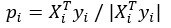
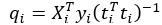
PLS regression identifies the normalized dimensions and that maximize the covariance between paired observations and , respectively. In our case, the visual stimulus is represented by a single variable , simplifying the problem to identifying the subspace of neural activity that optimally preserves information about the visual stimulus (sometimes referred to as PLS1 regression). That is, the N x T neural time series matrix X is reduced to a d x T matrix spanned by a set of orthonormal vectors. PLS1 regression is performed as follows:

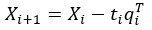
PLS1 algorithm

Let X_i = X and . For i = 1…d,

(1)

(2)

(3)

(4)

(5) 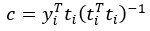(note this is scalar)

(6)

The projections of the neural data {p_i} thus span a subspace that maximally preserves information about the visual stimulus . Stacking these projections into the N x d matrix P that represents the transform from the whole-brain neural state space to the visually-evoked subspace, the optimal decoding direction is given by the linear least squares solution 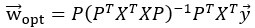. The dimensionality d of PLS regression was optimized using 6-fold cross-validation with 3 repeats and choosing the dimensionality between d = 1 and 20 with the lowest cross-validated mean squared error for each larva. Then, was computed using all time points.

For each stimulus type, the noise covariance matrix was computed in the low-dimensional PLS space, given that direct estimation of the noise covariances across many thousands of neurons would likely be unreliable. A noise covariance matrix was calculated separately for each stimulus, and then averaged across all stimuli. As before, the mean activity µ_i for each neuron was computed over each stimulus presentation period. The noise covariance then describes the correlated fluctuations δ_i around this mean response for each pair of neurons i and j, where

The noise modes for α = 1 …d were subsequently identified by eigendecomposition of the mean noise covariance matrix across all stimuli, . The angle between the optimal stimulus decoding direction and the noise modes is thus given by .”

- No response: It is not clear from the methods description if cases where the animal has no tail response are being lumped with cases where the animal decides to swim forward and thus has a large absolute but small mean tail curvature. These should be treated separately.

We thank the reviewer for raising the potential for this confusion and agree that forward-motion trials should not treated the same as motionless trials. While these types of trial were indeed treated separately in our original manuscript, we have updated the Methods section of our revised manuscript to make this clear:

“Left and right turn trials were extracted as described previously. Response trials included both left and right turn trials (i.e., the absolute value of mean tail curvature > σ_active), whereas nonresponse trials were motionless (absolute mean tail curvature < σ_active). In particular, forward-motion trials were excluded from these analyses.”

While our study has focused specifically on left and right turns, we hypothesize that the responsiveness bias ensemble may also be involved in forward movements and look forward to future work exploring the relationship between whole-brain dynamics and the full range of motor outputs.

- Behavioral variability: Related to Figure 2, within- and across-subject variability are confounded. Please disambiguate. It may also be informative on a per-fish basis to examine associations between reaction time and body movement.

The reviewer is correct that our previously reported summary statistics in Figure 2D-F were aggregated across trials from multiple larvae. Following the reviewer’s suggestion to make the magnitudes of across-larvae and within-larva variability clear, in our revised manuscript we have added two additional figure panels to Figure S2.

New Figure S2A highlights the across-larvae variability in mean head-directed behavioral responses to stimuli of various sizes. Overall, the relationship between stimulus size and the mean tail curvature across trials is largely consistent across larvae; however, the crossing-over point between leftward (positive curvature) and rightward (negative curvature) turns for a given side of the visual field exhibits some variability across larvae.

New Figure S2B shows examples of within-larva variability by plotting the mean tail curvature during single trials for two example larvae. Consistent with Figure 2G which also demonstrates within-larva variability, responses to a given stimulus are variable across trials in both examples. However, this degree of within-larva variability can appear different across larvae. For example, the larva shown on the left of Figure S2B exhibits greater overlap between responses to stimuli presented on opposite visual fields, whereas the larva shown on the right exhibits greater distinction between responses.

- Data presentation clarity: All figure panels need scale bars - for example, in Figure 3A there is no indication of timescale (or time of stimulus presentation). Figure 3I should also show the time series of the w_opt projection.

We appreciate the reviewer’s attention to detail in this regard. We have added scalebars to Figures 3A, 3H-I, S4B(ii), 4H, 4J in the revised manuscript, and all new figure panels where relevant. In addition, the caption of Figure 3A has been updated to include a description of the time period plotted relative to the onset of the visual stimulus.

Additionally, we appreciate the reviewer’s idea to show w_opt in Figure 3J of the revised manuscript (previously Figure 3I). This clearly shows that the visual decoding project is inactive during the short baseline period before visual stimulation begins, whereas the noise mode is correlated with motor output throughout the recording.

- Pixel locations: Given the poor quality of the brain images, it is difficult to tell the location of highlighted pixels relative to brain anatomy. In addition, given that the midbrain consists of much more than the tectum, it is not appropriate to put all highlighted pixels from the midbrain under the category of tectum. To aid in data interpretation and better connect this work with the literature, it is recommended that the authors register their data sets to standard brain atlases and determine if there is any clustering of relevant pixels in regions previously associated with prey-capture or predator-avoidance behavior.

We agree with the reviewer that registration of our datasets to a standard brain atlas is a highly useful addition. While the dense, pan-neuronal labeling makes the isolation of highly specific circuit components difficult, we have shown in more detail the specific brain regions contributing to these populations by aligning our recordings to the Z-Brain atlas (Randlett et al., 2015) as shown in new Figures S1E, S3F-G, 4I, 4K, and S5F-G. In addition, we provided a more detailed parcellation of the neuronal ensembles by providing projections of the full 3D volume along the xy and yz axes, in addition to the unregistered xy projection shown in new Figures 4H and 4J. We also found that the distribution of neurons in our huc:H2B-GCaMP6s recordings is very similar to the distribution of labeling in the huc:H2B-RFP reference image from the Z-Brain atlas (new Figure S1E), which further supports our whole-brain imaging results.

Overall, we find that this more detailed quantification and visualization is consistent with the interpretations in the previous version of our manuscript. In particular, we show that optimal visual decoding population (w_opt) and largest noise mode (e1) are localized to the midbrain (new Figures S3F-G), which is expected since in Figure 3 we first extracted a low-dimensional subspace of whole-brain neural activity that optimally preserved visual information. Additionally, we provide additional evidence that the populations correlated with the turn bias and responsiveness bias are distributed throughout the brain, including a relatively dense localization to the cerebellum, telencephalon, and dorsal diencephalon (habenula, new Figures 4H-K and S5F-G).

Finally, the reviewer is correct that our original label of “tectum” was a misnomer; the region analyzed corresponded to the midbrain, including the tegmentum, torus longitudinalis, and torus semicicularis in addition to the tectum. We have updated the brain regions shown and labels throughout the manuscript.

Interpretation

- W_opt and e_1 orthogonality: The statement that these two vectors, determined from analysis of the fluorescence data, are orthogonal, actually brings into question the idea that true signal and leading noise vectors in firing-rate state-space are orthogonal. First, the current analysis is confounding signals across different time periods - one could assume linearity all the way through the transformations, but this would only work if earlier sources of activation were being accounted for. Second, the transformation between firing rate and fluorescence is most likely not linear for GCaMP6s in most of the cells recorded. Thus, one would expect a change in the relationship between these vectors as one maps from fluorescence to firing rate.

Unfortunately, we are not entirely sure we have understood the reviewer’s argument. We are assuming that the reviewer’s first sentence is suggesting that the observation of orthogonality in the neural state space measured in calcium imaging precludes the possibility (“actually brings into question”, as the reviewer states) that the same neural ensembles could be orthogonal in firing rate state space measured by electrophysiological data. If this is the reviewer’s conjecture, we respectfully disagree with it. Consider a toy example of a neural network containing N ensembles of neurons, where the neurons within an ensemble all fire simultaneously, and two populations never fire at the same time. As long as the “switching” of firing between ensembles is not fast relative to the resolution of the GCaMP kernel, the largest principal components would represent orthogonal dimensions differentiating the various ensembles, both when observing firing rates or observing timeseries convolved by the GCaMP kernel. This is a simple example where the observed orthogonality would appear similar in both calcium imaging and electrophysical data, demonstrating that we should not allow conclusions from fluorescence data to “bring into question” that the same result could be observed in firing rate data.

We also disagree with the reviewer’s argument that we are “confounding signals across time periods”. Indeed, we must interpret the data in light of the GCaMP response kernel. However, all of the analyses presented here are performed on instantaneous measurements of population activity patterns. These activity patterns do represent a smoothed, likely nonlinear integration of recent neuronal activity, but unless the variability in the GCaMP response kernel (discussed above) is widely different across these populations (which has not been observed in the literature), we do not expect that the GCaMP transformations would artificially induce orthogonality in our analysis approach. Such smoothing operations tend to instead increase correlations across neurons and population decoding approaches generally benefit from this smoothness, as we have argued above. However, a much more problematic situation would be if we were comparing the activity of two neuronal populations at different points in time (which we do not include in this study), in which case the nonlinearities could overaccentuate orthogonality between non-time-matched activity patterns.

Finally, we agree with the reviewer that the transformation between firing rate and fluorescence is very likely nonlinear and that these vectors of population activity do not perfectly represent what would be observed if one had access to whole-brain, cellular-resolution electrophysiology spike data. However, similar observations regarding the brain-wide, distributed encoding of behavior have been confirmed across recording modalities in the mouse (Stringer et al., 2019; Steinmetz et al., 2019), where large-scale electrophysiology utilizing highly invasive probes (e.g., Neuropixels) is more feasible than in the larval zebrafish. With the advent of whole-brain voltage imaging in the larval zebrafish, we expect any differences between calcium and voltage dynamics will be better understood, yet such techniques will likely continue to suffer to some extent from the nonlinearities described here.

- Sources of variability: The authors do not take into account a fairly obvious source of variability in trial-to-trial response - eye position. We know that prey capture responsiveness is dependent on eye position during stimulus (see Figure 4 of PMID: 22203793). We also expect that neurons fairly early in the visual pathway with relatively narrow receptive fields will show variable responses to visual stimuli as the degree of overlap with the receptive field varies with eye movement. There can also be small eye-tracking movements ahead of the decision to engage in prey capture (Figure 1D, PMID: 31591961) that can serve as a drive to initiate movements in a particular direction. Given these possibilities indicating that the behavioral measure of interest is gaze, and the fact that eye movements were apparently monitored, it is surprising that the authors did not include eye movements in the analysis and interpretation of their data.

We agree with the reviewer that eye movements, such as saccades and convergence, are important motor outputs that are well-known to play a role in the sequence of motor actions during prey capture and other behaviors. Therefore, we have added the following new eye tracking results to our revised manuscript:

“In order to confirm that the observed neural variability in the visually-evoked populations was not predominantly due to eye movements, such as saccades or convergence, we tracked the angle of each eye. We utilized DeepLabCut, a deep learning tool for animal pose estimation (Mathis et al., 2018), to track keypoints on the eye which are visible in the raw fLFM images, including the retina and pigmentation (Figure S3D(i)). This approach enabled identification of various eye movements, such as convergence and the optokinetic reflex (Figure S3D(ii-iii)). Next, we extracted a number of various eye states, including those based on position (more leftward vs. rightward angles) and speed (high angular velocity vs. low or no motion). Figure S3E(i) provides example stimulus response profiles across trials of the same visual stimulus in each of these eye states, similar to a single column of traces in Figure 3A broken out into more detail. These data demonstrate that the magnitude and temporal dynamics of the stimulus-evoked responses show apparently similar levels of variability across eye states. If neural variability was driven by eye movement during the stimulus presentation, for example, one would expect to see much more variability during the high angular velocity trials than low, which is not apparent. Next, we asked whether the dominant neural noise modes vary across eye states, which would suggest that the geometry of neuronal variability is influenced by eye movements or states. To do so, the dominant noise modes were estimated in each of the individual eye conditions, as well as bootstrapped trials from across all eye conditions. The similarity of these noise modes estimated from different eye conditions (Figure S3E(ii), right)) was not significantly different from the similarity of noise modes estimated from bootstrapped random samples across all eye conditions (Figure S3E(ii), left)). Therefore, while movements of the eye likely contribute to aspects of the observed neural variability, they do not dominate the observed neural variability here, particularly given our observation that the largest noise mode represents a considerable fraction of the observed neural variance (Figure 3E).”

While these results provide an important control in our study, we anticipate further study of the relationship between eye movements or states, visually-evoked neural activity, and neural noise modes would identify the additional neural ensembles which are correlated with and drive this additional motor output.

Reviewer #3 (Public Review):

Summary:

In this study, Manley and Vaziri designed and built a Fourier light-field microscope (fLFM) inspired by previous implementations but improved and exclusively from commercially available components so others can more easily reproduce the design. They combined this with the design of novel algorithms to efficiently extract whole-brain activity from larval zebrafish brains.

This new microscope was applied to the question of the origin of behavioral variability. In an assay in which larval zebrafish are exposed to visual dots of various sizes, the fish respond by turning left or right or not responding at all. Neural activity was decomposed into an activity that encodes the stimulus reliably across trials, a 'noise' mode that varies across trials, and a mode that predicts tail movements. A series of analyses showed that trial-to-trial variability was largely orthogonal to activity patterns that encoded the stimulus and that these noise modes were related to the larvae's behavior.

To identify the origins of behavioral variability, classifiers were fit to the neural data to predict whether the larvae turned left or right or did not respond. A set of neurons that were highly distributed across the brain could be used to classify and predict behavior. These neurons could also predict spontaneous behavior that was not induced by stimuli above chance levels. The work concludes with findings on the distributed nature of single-trial decision-making and behavioral variability.

Strengths:

The design of the new fLFM microscope is a significant advance in light-field and computational microscopy, and the open-source design and software are promising to bring this technology into the hands of many neuroscientists.

The study addresses a series of important questions in systems neuroscience related to sensory coding, trial-to-trial variability in sensory responses, and trial-to-trial variability in behavior. The study combines microscopy, behavior, dynamics, and analysis and produces a well-integrated analysis of brain dynamics for visual processing and behavior. The analyses are generally thoughtful and of high quality. This study also produces many follow-up questions and opportunities, such as using the methods to look at individual brain regions more carefully, applying multiple stimuli, investigating finer tail movements and how these are encoded in the brain, and the connectivity that gives rise to the observed activity. Answering questions about variability in neural activity in the entire brain and its relationship to behavior is important to neuroscience and this study has done that to an interesting and rigorous degree.

Points of improvement and weaknesses:

The results on noise modes may be a bit less surprising than they are portrayed. The orthogonality between neural activity patterns encoding the sensory stimulus and the noise modes should be interpreted within the confounds of orthogonality in high-dimensional spaces. In higher dimensional spaces, it becomes more likely that two random vectors are almost orthogonal. Since the neural activity measurements performed in this study are quite high dimensional, a more explicit discussion is warranted about the small chance that the modes are not almost orthogonal.

We agree with the reviewer that orthogonality is less “surprising” in high-dimensional spaces, and we have added this important point of interpretation to our revised manuscript. Still, it is important to remember that while the full neural state space is very high-dimensional (we record that activity of up to tens of thousands of neurons simultaneously), our analyses regarding the relationship between the trial-to-trial noise modes and decoding dimensions were performed in a low-dimensional subspace (up to 20 dimensions) identified by PLS regression to that optimally preserved visual information. This is a key step in our analysis which serves two purposes: 1. it removes some of the confound described the reviewer regarding the dimensionality of the neural state space analyzed; and 2. it ensures that the noise modes we analyze are even relevant to sensorimotor processing. It would certainly not be surprising or interesting if we identified a neural dimension outside the midbrain which was orthogonal to the optimal visual decoding dimension.

Regardless, in order to better control for this confound, we estimated the distribution of angles between random vectors in this subspace. As we describe in the revised manuscript:

“However, in high-dimensional spaces, it becomes increasingly common that two random vectors could appear orthogonal. While this is particularly a concern when analyzing a neural state space spanned by tens of thousands of neurons, our application of PLS regression to identify a low-dimensional subspace of relevant neuronal activity partially mitigates this concern. In order to control for this confound, we compared the angles between w_opt and e1 across larvae to that computed with shuffled versions of w_opt,shuff estimated by randomly shuffling the stimulus labels before identifying the optimal decoding direction. While it is possible to observe shuffled vectors which are nearly orthogonal to e₁, the shuffled distribution spans a significantly greater range of angles than the observed data, demonstrating that this orthogonality is not simply a consequence of analyzing multi-dimensional activity patterns.”

The conclusion that sparsely distributed sets of neurons produce behavioral variability needs more investigation because the way the results are shown could lead to some misinterpretations. The prediction of behavior from classifiers applied to neural activity is interesting, but the results are insufficiently presented for two reasons.

(1) The neurons that contribute to the classifiers (Figures 4H and J) form a sufficient set of neurons that predict behavior, but this does not mean that neurons outside of that set cannot be used to predict behavior. Lasso regularization was used to create the classifiers and this induces sparsity. This means that if many neurons predict behavior but they do so similarly, the classifier may select only a few of them. This is not a problem in itself but it means that the distributions of neurons across the brain (Figures 4H and J) may appear sparser and more distributed than the full set of neurons that contribute to producing the behavior. This ought to be discussed better to avoid misinterpretation of the brain distribution results, and an alternative analysis that avoids the confound could help clarify.

We thank the reviewer for raising this point, which we agree should be discussed in the manuscript. Lasso regularization was a key ingredient in our analysis; l2 regularization alone was not sufficient to prevent overfitting to the training trials, particularly when decoding turn direction and responsiveness. Previous studies have also found that sparse subsets of neurons better predict behavior than single neuron or non-sparse populations, for example Scholz et al. (2018).

While showing l2 regularization would not be a fair comparison given the poor performance of the l2-regularized classifiers, we opted to identify a potentially “fuller” set of neurons correlated with these biases based on the correlation between each neuron’s activity over the recording and the projection along the turn direction or responsiveness dimension identified using l1 regularization. This procedure has the potential to identify all neurons correlated with the final ensemble dynamics, rather than just a “sufficient set” for lasso regression. In new Figures S5F-G, we show the 3D distribution of all neurons significantly correlated with these biases, which appear similar to those in Figures 4H-K and widely distributed across practically the entire labeled area of the brain.

(2) The distribution of neurons is shown in an overly coarse manner in only a flattened brain seen from the top, and the brain is divided into four coarse regions (telencephalon, tectum, cerebellum, hindbrain). This makes it difficult to assess where the neurons are and whether those four coarse divisions are representative or whether the neurons are in other non-labeled deeper regions. For these two reasons, some of the statements about the distribution of neurons across the brain would benefit from a more thorough investigation.

We agree with the reviewer that a more thorough description and visualization of these distributed populations is warranted.

While the dense, pan-neuronal labeling makes the isolation of highly specific circuit components difficult, we have shown in more detail the specific brain regions contributing to these populations by aligning our recordings to the Z-Brain atlas (Randlett et al., 2015) as shown in new Figures S1E, S3F-G, 4I, 4K, and S5F-G. In addition, we provided a more detailed parcellation of the neuronal ensembles by providing projections of the full 3D volume along the xy and yz axes, in addition to the unregistered xy projection shown in new Figures 4H and 4J. We also found that the distribution of neurons in our huc:H2B-GCaMP6s recordings is very similar to the distribution of labeling in the huc:H2B-RFP reference image from the Z-Brain atlas (new Figure S1E), which further supports our whole-brain imaging results.

Overall, we find that this more detailed quantification and visualization is consistent with the interpretations in the previous version of our manuscript. In particular, we show that optimal visual decoding population (w_opt) and largest noise mode (e1) are localized to the midbrain (new Figures S3F-G), which is expected since in Figure 3 we first extracted a low-dimensional subspace of whole-brain neural activity that optimally preserved visual information. Additionally, we provide additional evidence that the populations correlated with the turn bias and responsiveness bias are distributed throughout the brain, including a relatively dense localization to the cerebellum, telencephalon, and dorsal diencephalon (habenula, new Figures 4H-K and S5F-G).

Recommendations for the authors:

Reviewer #1 (Recommendations For The Authors):

In addition to the overall strengths and weaknesses above, I have a few specific comments that I think could improve the study:

(1) In lines 334-335 you write that 'We proceeded to build various logistic regression classifiers to decode'. Do you mean you tested this with other classifier types as well (e.g. SVM, Naive Bayes) or do you mean various because you trained the classifier described in the methods on each animal? This is not clear. If it is the first, more information is needed about what other classifiers you used.

We appreciate the reviewer raising this point of clarification. Here, we simply meant that we fit the multiclass logistic regression classifier in the one-vs-rest scheme. In this sense, a single multiclass logistic regression classifier was fit for each larva. We have updated our revised manuscript with this clarification: “The visual stimuli were decoded using a one-versus-rest, multiclass logistic regression classifier with lasso regularization.”

(2) In Figure 3 you train the decoder on all visually responsive cells identified across the brain. Does this reliability of stimulus decoding also hold for neurons sampled from specific brain regions? For example, does this reliable decoding come from stronger and more reliable responses in the optic tectum, whereas stimulus decodability is not as good in visual encoding neurons identified in other structures?

In new Figure S5B, we show the performance of stimulus decoding from various brain regions. We find that stimulus classification is possible from the midbrain and cerebellum, very poor from the hindbrain, and not possible from the telencephalon during the period between stimulus onset and the decision.

(3) In relation to point 2, it would be good to show in which brain areas the visually responsive neurons are located, and maybe the average coefficients per brain area. Plots like Figures 3G, and H would benefit from a quantification into areas. Similarly, a parcellation into more specific brain areas in Figure 4 would also be valuable.

In addition to providing a more detailed parcellation of the turn direction and responsiveness bias populations in Figure 4, we have provided a similar visualization and quantification of the optimal stimulus decoding population and the dominant noise mode in new Figures S3F-G, respectively.

(4) In Figure 3f, it is not clear to me how this shows that w_opt and e1 are orthogonal. They appear correlated.

The orthogonality we quantify is related to the pattern of coefficients across neurons, not necessarily the timeseries of their projections. The slight shift in the noise mode activations as you move from stimuli on the left visual field to the right actually comes from the motor outputs. Large left stimuli tend to evoke a rightward turn and vice versa, and the example noise mode shown encodes the directionality and vigor of tail movements, resulting in the slight shifts observed.

(5) I think the wording of this conclusion is too strong for the results and a bit illogical:

'Thus, our data suggest that the neural dynamics underlying single-trial action selection are the result of a widely-distributed circuit that contains subpopulations encoding internal time-varying biases related to both the larva's responsiveness and turn direction, yet distinct from the sensory encoding circuitry.'

If that is the case, how is it even possible that the larvae can do a visually guided behaviour?

Especially given Suppl Fig 4C it would be more appropriate to say something along the lines of: 'When stimuli are highly ambiguous, single trial action selection is dominated by widely-distributed circuit that contains subpopulations encoding internal time-varying biases related to both the larva's responsiveness and turn direction, that encode choice distinctly from the sensory encoding circuitry'.

We appreciate the reviewer’s suggestion and have re-worded this line in the discussion in order to clarify that these time-varying biases are predominant in the case of ambiguous stimuli, as shown in Figure S5C in our revised manuscript (corresponding to Figure S4C in our original submission).

(6) Line 599: typo: trial-to-trail

We thank the reviewer for noting this error, which has been corrected in the revised text of the manuscript.