Flagellar synchronization through direct hydrodynamic interactions
- University of Cambridge, United Kingdom
- Massachusetts Institute of Technology, United States
- University of Warwick, United Kingdom
Figures
Figure 1 with 1 supplement

Synchronized pairs of beating flagella.
(A) Experimental apparatus and (B) cell configuration. (C) Extracted phase difference at four different interflagellar spacings, as indicated. These separations correspond to scaled spacing L = d/l of 0.85, 1.22, 1.69, and 2.27. (D) fluctuations during phase-locked periods around the average phase lag, Δ0, and (E) the fluctuations’ probability distribution functions (PDFs), each cast in terms of the rescaled separation-specific variable (Δ − Δ0)/√L. Solid lines represent Gaussian fits. Further details of the phase extraction procedure can be found in Figure 1—figure supplement 1. Samples of the four processed videos corresponding to the cells in Figure 1C are shown in Video 1.
Figure 1—figure supplement 1
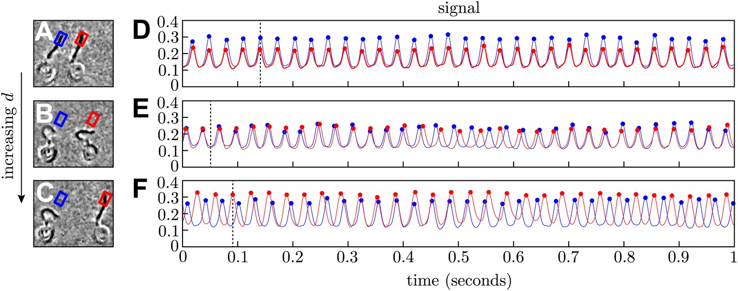
Phase extraction.
(A–C) Snapshots from three different processed videos showing the same cells at different interflagellar spacings (d = 14.2, 20.4, 28.2 μm). (D–F) The signal extracted from the interrogation regions is used to reconstruct the flagellar phases. For each row, the frame on the left corresponds to the time indicated by the dashed line.
Figure 2
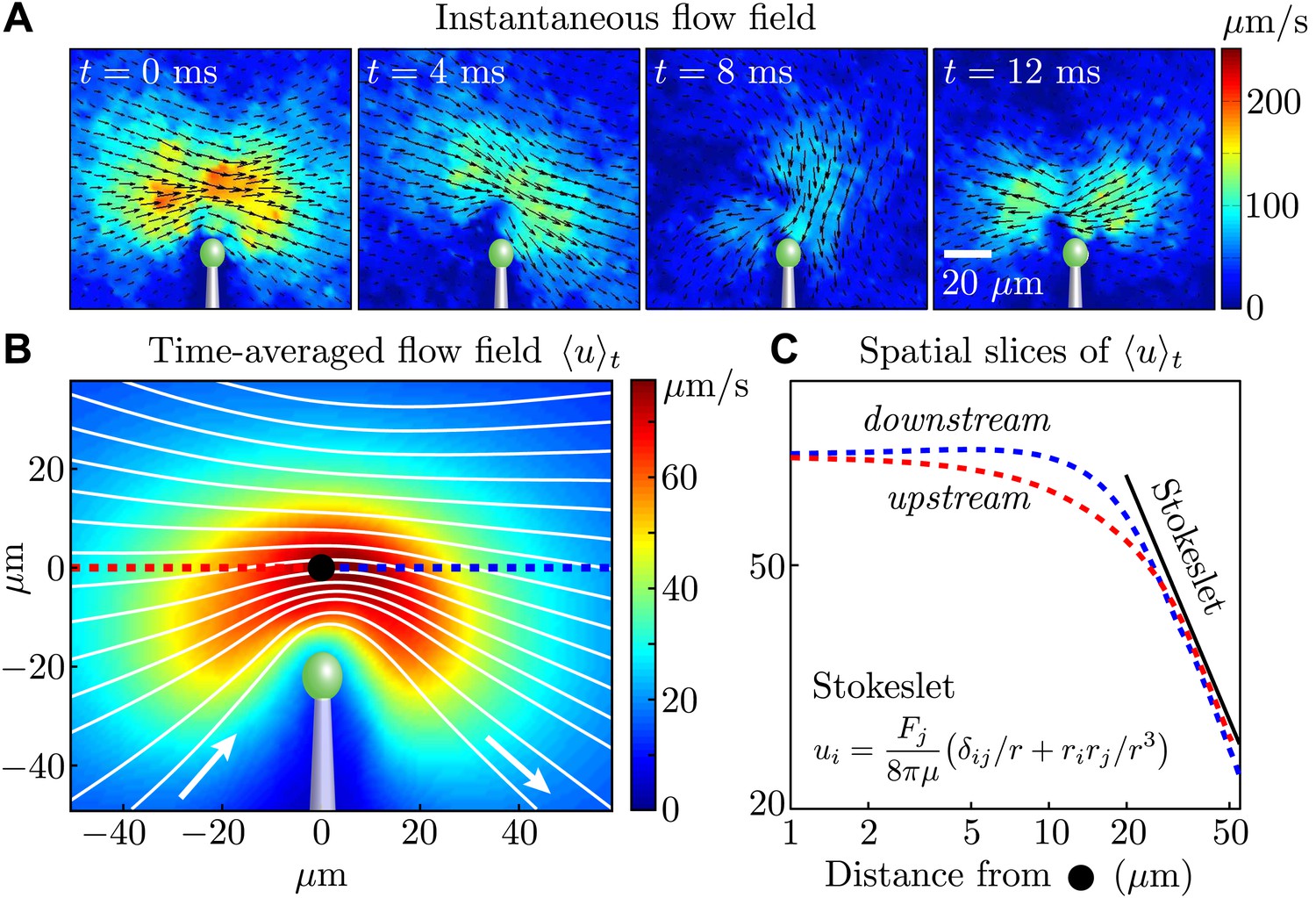
Measured flagellar flow field.
(A) Time-dependent flow field for an individual cell measured using particle image velocimetry. Results are shown for the first half of the beating cycle. (B) Time-averaged flow field (averaged across 4 cells with τ ∼ 1000 beats for each). The velocity magnitude (colour) and streamlines (white) are shown. (C) Velocity magnitude upstream (red) and downstream (blue) of the origin (black dot in B).
Figure 3 with 1 supplement
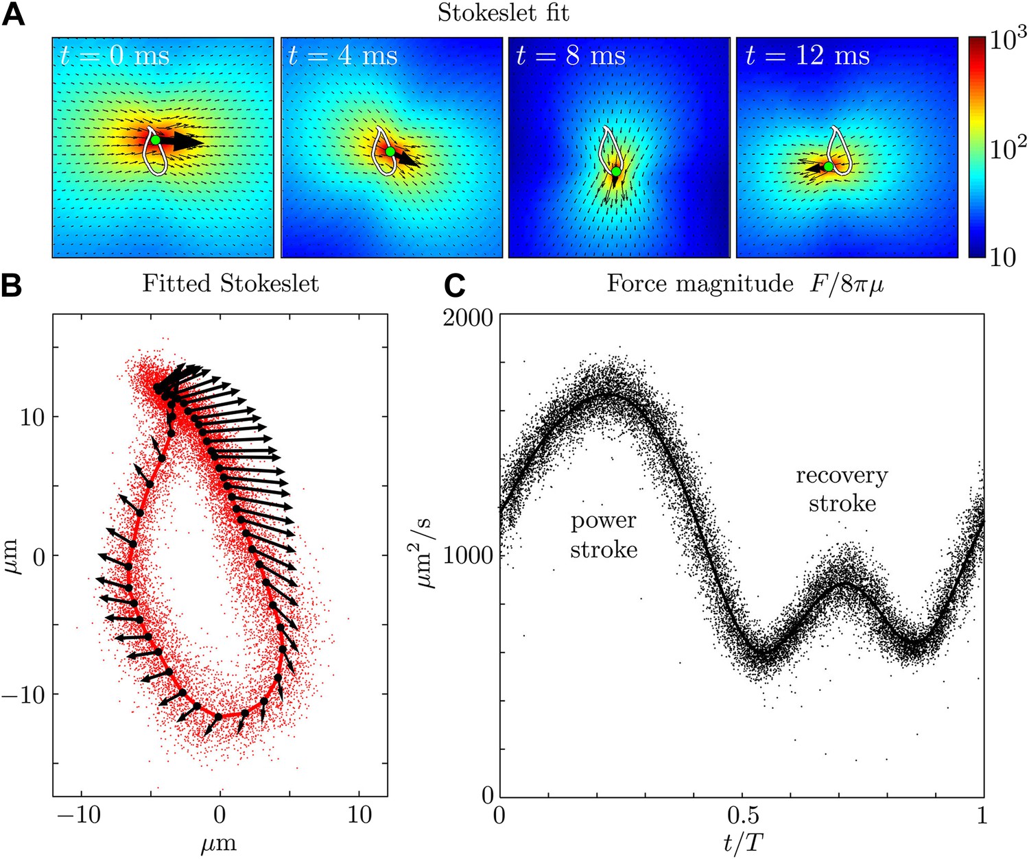
Force amplitude of flagellum.
(A) Fitted instantaneous velocity field at various stages during the first half of one representative flagellar beat. (B) The fitted Stokeslet is shown at evenly-spaced times throughout the average flagellar beat cycle. The red dots indicate the Stokeslet position extracted from every frame. (C) Amplitude of the fitted point force as a function of time throughout the flagellar beat period T.
Figure 3—figure supplement 1

Time-dependent flow fields.
Instantaneous fluid velocity corresponding to various stages during one representative flagellar beat. Also shown are the fitted flow fields for each frame, corresponding to the application of a point force on the fluid. Very good qualitative agreement can be seen.
Figure 4
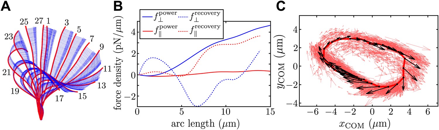
Resistive force theory analysis.
(A) Instantaneous velocity distribution along the flagellum during one complete beat cycle (indexed by frame number, imaged at 1000 fps). (B) Components of integrated force density produced by a flagellum executing characteristic power and recovery strokes, as a function of arclength along the flagellum measured from the basal to the distal end. (C) Integrated vector forces F(t) shown localised at centre-of-mass coordinates x(t) (red: per frame, black: averaged over O(103) frames), evolve cyclically around an average trajectory. The average value is |F|/8πμ ∼ 1910 μm2/s.
Figure 5
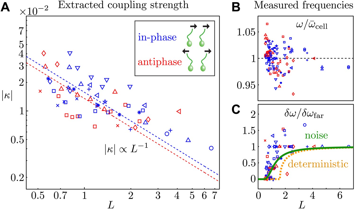
Coupling strength.
(A) Dimensionless interflagellar coupling strength as a function of the scaled spacing L = d/l (log–log scale). The dotted lines represent fits of the form with k = 0.016 (in-phase) and k = 0.014 (antiphase). (B) Measured beat frequency of each flagellum, nondimensionalised by the average value for that cell across several videos. (C) Measured frequency difference as a function of spacing L. The curves represent the predictions based on the average extracted model parameters in the absence (orange) and presence of noise (green). Symbols represent different pairs of cells, with the in-phase (blue) and antiphase (red) configurations shown.
Figure 6 with 2 supplements
Waveform characteristics.
(A) Logarithmically-scaled residence time plots of the entire flagella. The displayed waveforms correspond to 1 ms time intervals over several successive flagellar beats. (B) Angles xa, xb, xc (in radians) measured and (C) their characteristic 3D trajectories. Results are shown for the right flagellum, corresponding to three different interflagellar spacings. As the spacing d is increased, the flagellar waveform exhibits a systematic change.
Figure 6—figure supplement 1
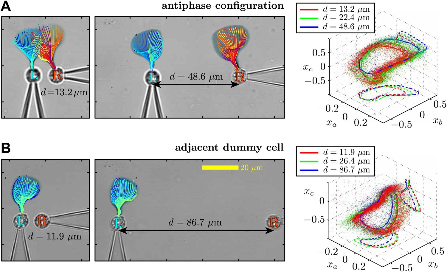
Flagellar filaments are tracked for cells in the (A) antiphase state, as well as (B) the situation in which one of the cells does not possess a flagellum (dummy cell).
For each configuration, the waveform of the left cell is analysed at three different cell–cell separations.
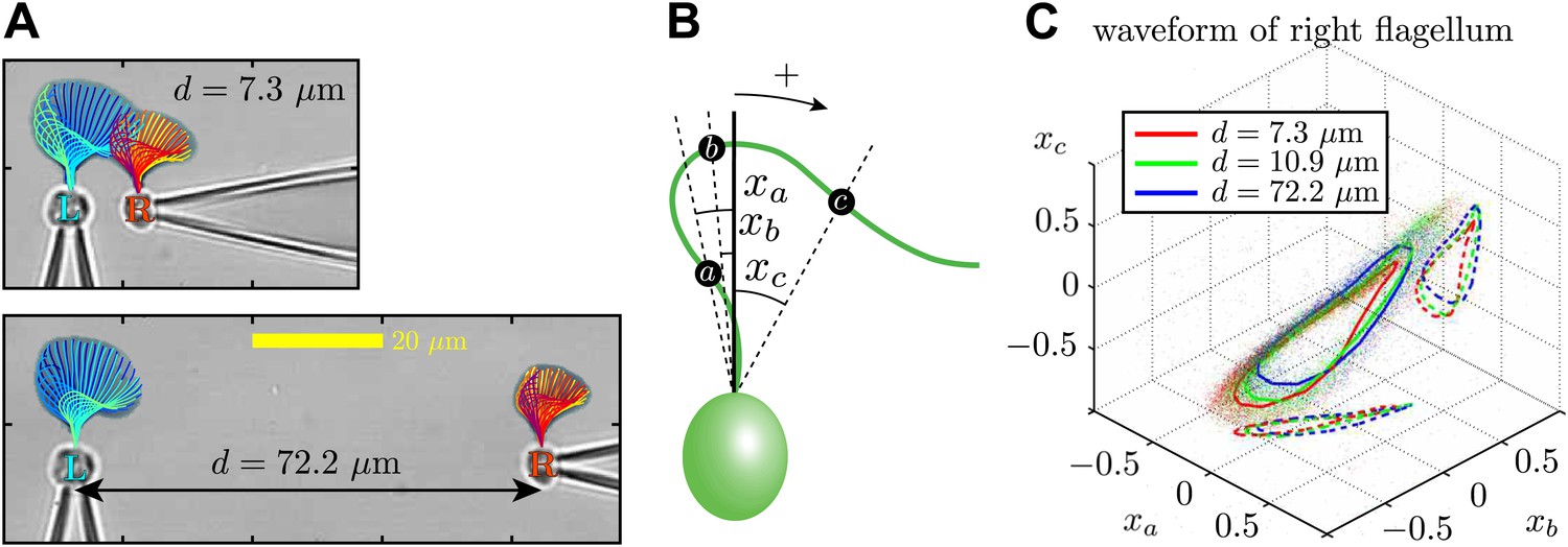
Figure 6—figure supplement 2
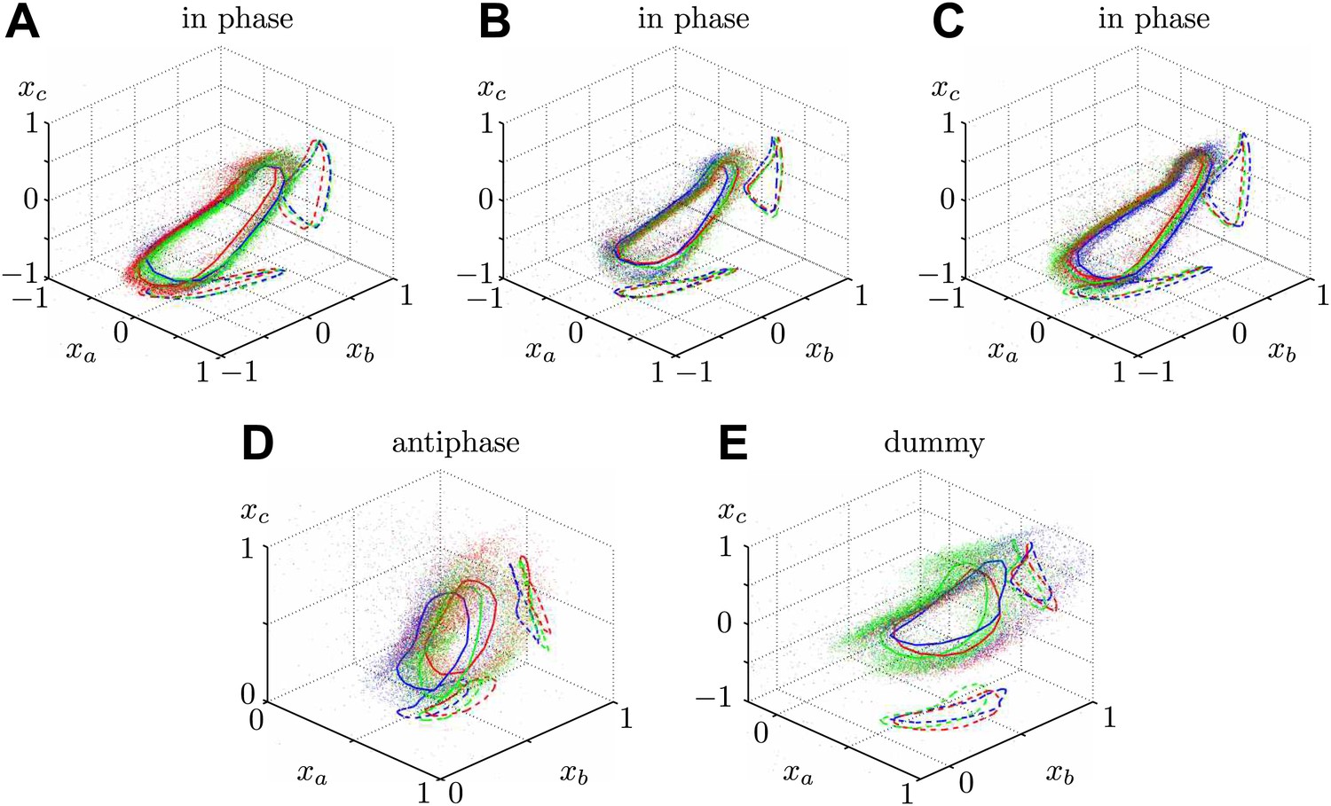
Additional waveform data collected for 5 different cells in various geometric configurations.
The colours RGB correspond to increasing inflagellar spacing respectively, with distances (in micrometres) given by (A) {7.3, 10.9, 72.2}, (B) {6.5, 11.0, 27.1}, (C) {9.2, 14.2, 34.7}, (D) {10.3, 31.0, 84.0}, (E) {12.1, 16.2, 67.3}.
Figure 7
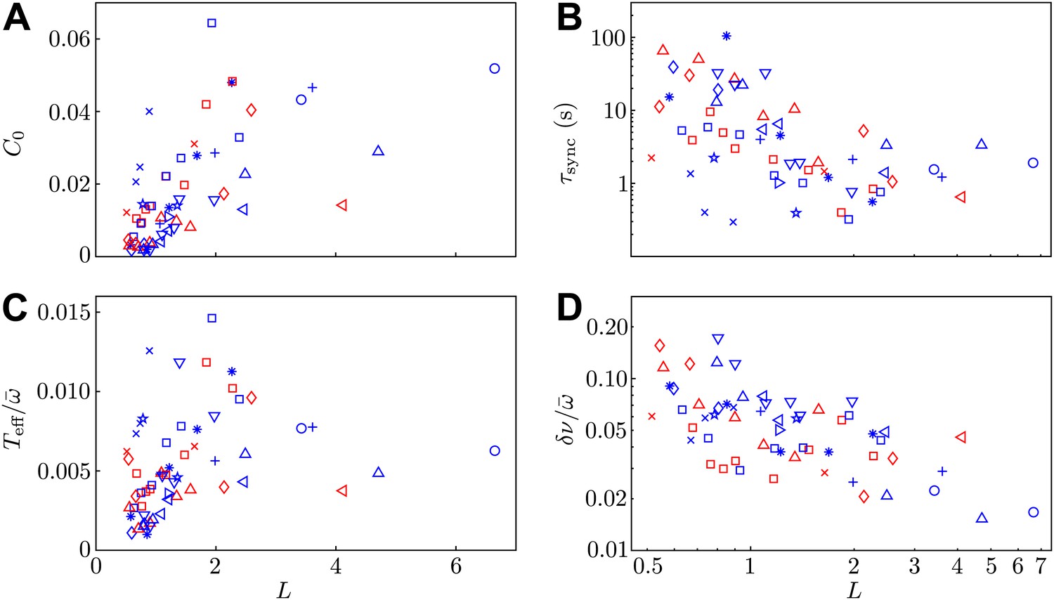
Model parameters.
Two of the experimental observables (A) C0 and (B) , and the two additional model parameters (C) and (D) are shown as functions of interflagellar spacing for all experiments conducted.
Figure 8
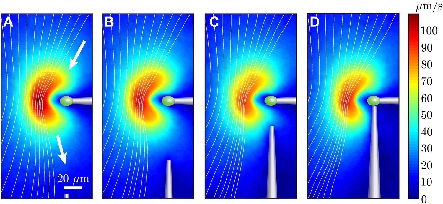
Effect of nearby pipette.
The time-averaged flow field associated with one captured cell is measured as a second pipette slowly approaches. This demonstrates that the precise angle from which the cell is held by the micropipette has very little effect on the resultant flow field.
Figure 9
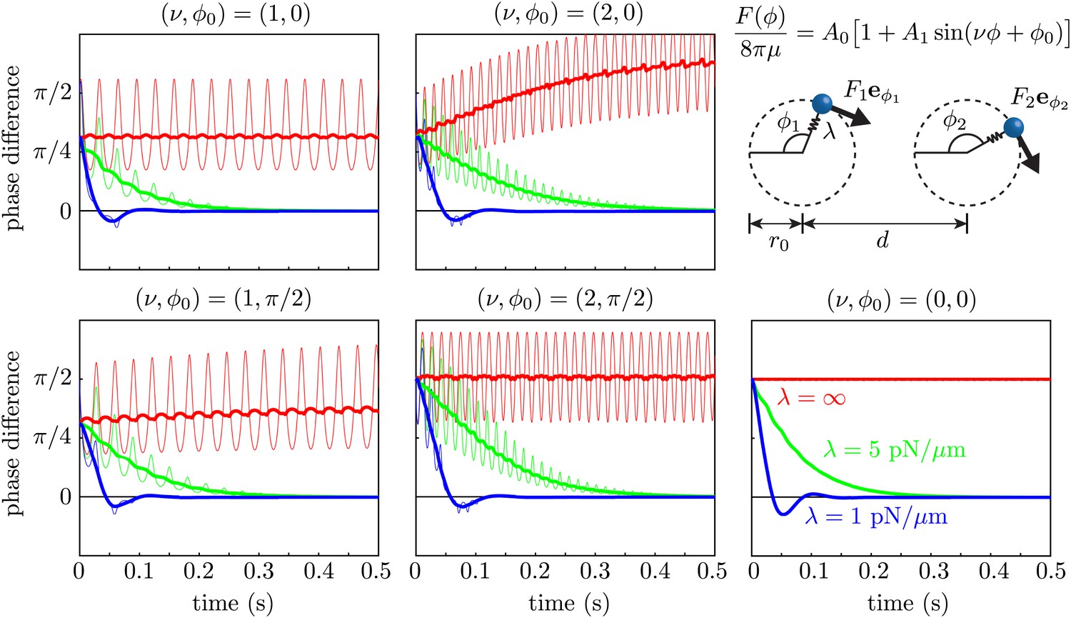
Effect of force modulation.
Evolution of the phase difference among two identical model oscillators, each composed of a sphere driven around a circular trajectory by a tangential driving force. The trajectories each possess a radial stiffness λ. Smaller values of λ yield rapid convergence towards synchrony (δ = 0), in a manner essentially independent of the functional form of the driving force. Parameters used are given by a = 0.75 μm, r0 = 8 μm, d = 20 μm, A0 = 1076 μm2/s and A1 = 0.56.
Figure 10
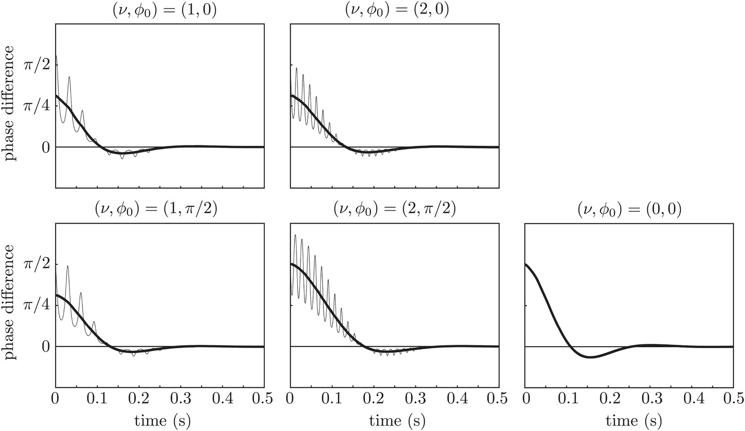
Effect of force modulation.
Re-run of the simulations in Figure 9 with properties inspired by real flagella.
Videos
Video 1
A pair of hydrodynamically coupled flagella, observed at various cell–cell spacings.
Original videos were recorded at 1000 fps, with processed representative segments (1000 frames each) replayed here at 25 fps.
Video 2
Experiments in which one cell does not possess a flagellum.
Figures (A and B) and (C and D) correspond to two different pairs of cells respectively. In each case, the flagellated cell exhibits some counterrotation during the beating, while the 'dummy cell' subject to the flow displays no visible rocking. Videos were recorded at 1000 fps and are replayed here at 25 fps.
Download links
A two-part list of links to download the article, or parts of the article, in various formats.
Downloads (link to download the article as PDF)
Open citations (links to open the citations from this article in various online reference manager services)
Cite this article (links to download the citations from this article in formats compatible with various reference manager tools)
Flagellar synchronization through direct hydrodynamic interactions
eLife 3:e02750.
https://doi.org/10.7554/eLife.02750


