Optimal multisensory decision-making in a reaction-time task
- University of Rochester, United States
- Institut National de la Santé et de la Recherche Médicale, École Normale Supérieure, France
- Université de Genève, Switzerland
- Baylor College of Medicine, United States
Figures
Figure 1
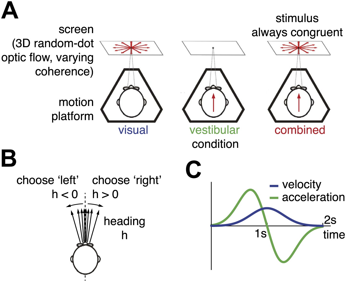
Heading discrimination task.
(A) Subjects are seated on a motion platform in front of a screen displaying 3D optic flow. They perform a heading discrimination task based on optic flow (visual condition), platform motion (vestibular condition), or both cues in combination (combined condition). Coherence of the optic flow is constant within a trial but varies randomly across trials. (B) The subjects' task is to indicate whether they are moving rightward or leftward relative to straight ahead. Both motion direction (sign of h) and heading angle (magnitude of ) are chosen randomly between trials. (C) The velocity profile is Gaussian with peak velocity ∼1 s after stimulus onset.
Figure 2 with 1 supplement
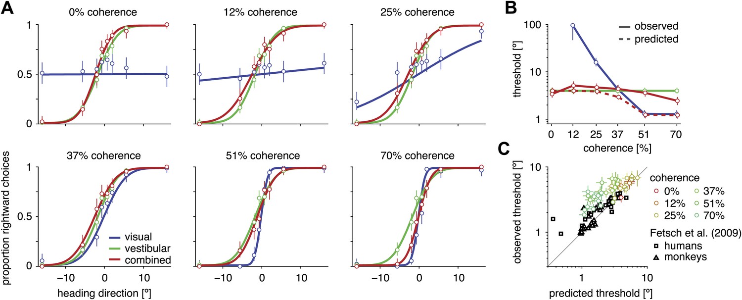
Heading discrimination performance.
(A) Plots show the proportion of rightward choices for each heading and stimulus condition. Data are shown for subject D2, who was tested with 6 coherence levels. Error bars indicate 95% confidence intervals. (B) Discrimination threshold for each coherence and condition for subject D2 (see Figure 2—figure supplement 1 for discrimination thresholds of all subjects). For large coherences, the threshold in the combined condition (solid red curve) lies between that of the vestibular and visual conditions, a marked deviation from the standard prediction (dashed red curve) of optimal cue integration theory. (C) Observed vs predicted discrimination thresholds for the combined condition for all subjects. Data are color coded by motion coherence. Error bars indicate 95% CIs. For most subjects, observed thresholds are significantly greater than predicted, especially for coherences greater than 25%. For comparison, analogous data from monkeys and humans (black triangles and squares, respectively) are shown from a previous study involving a fixed-duration version of the same task (Fetsch et al., 2009).
Figure 2—figure supplement 1

Discrimination thresholds for all subjects and conditions.
The psychophysical thresholds are found by fitting a cumulative Gaussian function to the psychometric curve for each condition. The predicted threshold is based on the visual and vestibular thresholds measured at the same coherence. The error bars indicate bootstrapped 95% CIs. Note that the observed thresholds in the combined condition (solid red curves) are consistently greater than the predicted thresholds (dashed red curves), especially at high coherences. For a statistical comparison between various thresholds see Supplementary file 2A.
Figure 3 with 2 supplements
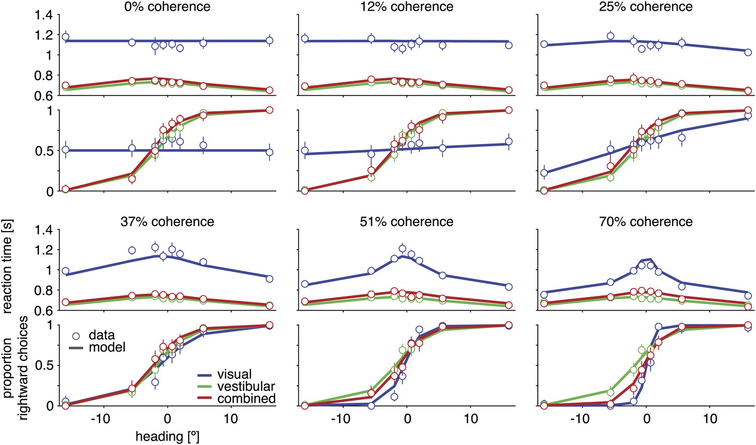
Discrimination performance and reaction times for subject D2.
Behavioral data (symbols with error bars) and model fits (lines) are shown separately for each motion coherence. Top plot: reaction times as a function of heading; bottom plot: proportion of rightward choices as a function of heading. Mean reaction times are shown for correct trials, with error bars representing two SEM (in some cases smaller than the symbols). Error bars on the proportion rightward choice data are 95% confidence intervals. Although reaction times are only shown for correct trials, the model is fit to data from both correct and incorrect trials. See Figure 3—figure supplement 1 for behavioral data and model fits for all subjects. Figure 3—figure supplement 2 shows the fitted model parameters per subject.
Figure 3—figure supplement 1
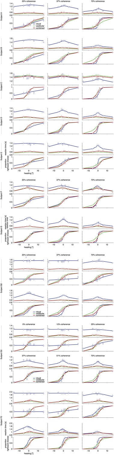
Psychometric functions, chronometric functions, and model fits for all subjects.
Behavioral data (symbols with error bars) and model fits (lines) are, for clarity, shown separately for each different coherence of the visual motion stimulus. The reaction time shown is the mean reaction time for correct trials, with error bars showing two SEMs (sometimes smaller than the symbols). Error bars on the proportion of rightward choices are 95% confidence intervals. Note that reaction times are shown only for correct trials, while the model is fit to both correct and incorrect trials.
Figure 3—figure supplement 2

Model parameters for fits of the optimal model and two alternative parameterizations.
Based on the maximum likelihood parameters of full model fits for each subject, the four top plots show how drift rate and normalized bounds are assumed to depend on visual motion coherence. The solid lines show fits for the model described in the main text. The dashed lines show fits for an alternative parameterization with one additional parameter (see Supplementary file 1). The circles show the fits of a model that, instead of linking them by a parametric function, fits these drifts and bounds for each coherence separately. As can be seen, the parametric functions qualitatively match these independent fits. The bottom bar graphs show drift rate and bound for the vestibular modalities and fitted non-decision times for each subject, all for the model parameterization described in the text. All error bars show ±1 SD of the parameter posterior. Each color corresponds to a separate subject, with color scheme given by the bottom left bar graph.
Figure 4
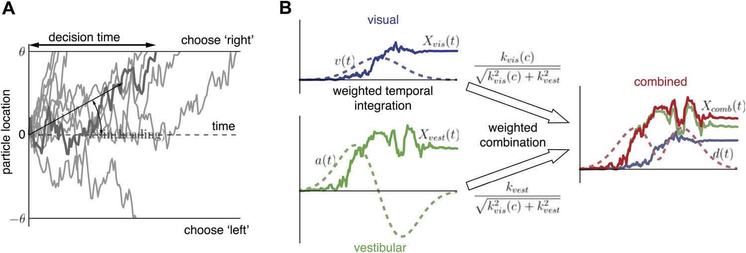
Extended diffusion model (DM) for heading discrimination task.
(A) A drifting particle diffuses until it hits the lower or upper bound, corresponding to choosing ‘left’ or ‘right’ respectively. The rate of drift (black arrow) is determined by heading direction. The time at which a bound is hit corresponds to the decision time. 10 particle traces are shown for the same drift rate, corresponding to one incorrect and nine correct decisions. (B) Despite time-varying cue sensitivity, optimal temporal integration of evidence in DMs is preserved by weighting the evidence by the momentary measure of its sensitivity. The DM representing the combined condition is formed by an optimal sensitivity-weighted combination of the DMs of the unimodal conditions.
Figure 5
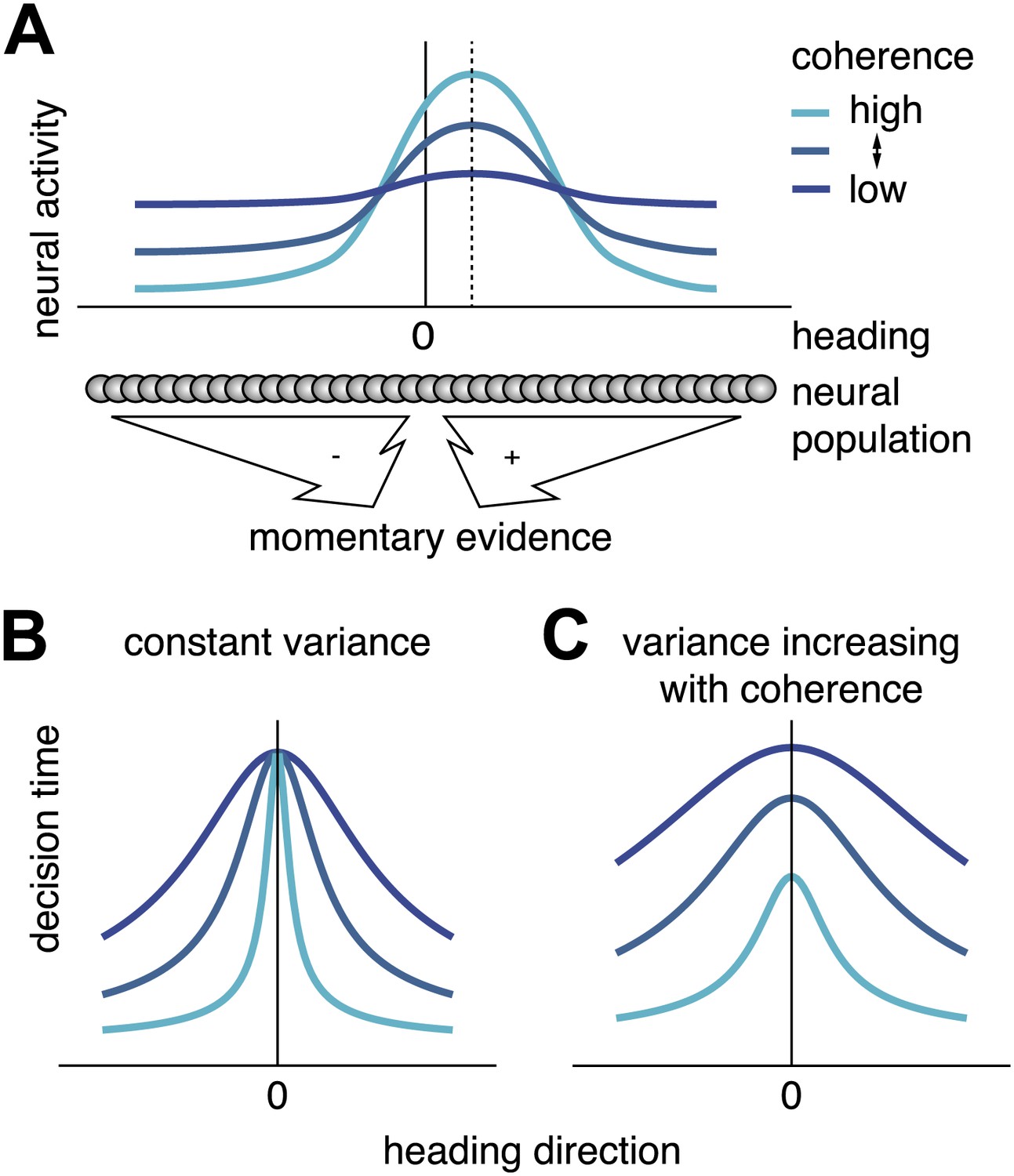
Scaling of momentary evidence statistics of the diffusion model (DM) with coherence.
(A) Assumed neural population activity giving rise to the DM mean and variance of the momentary evidence, and their dependence on coherence. Each curve represents the activity of a population of neurons with a range of heading preferences, in response to optic flow with a particular coherence and a heading indicated by the dashed vertical line. (B) Expected pattern of reaction times if variance is independent of coherence. If neither the DM bound nor the DM variance depend on coherence, the DM predicts the same decision time for all small headings, regardless of coherence. This is due to the DM drift rate, kvis(c)sin(h) being close to 0 for small headings, h≈0, independent of the DM sensitivity kvis(c). (C) Expected pattern of reaction times when variance scales with coherence. If both DM sensitivity and DM variance scale with coherence while the bound remains constant, the DM predicts different decision times across coherences, even for small headings. Greater coherence causes an increase in variance, which in turn causes the bound to be reached more quickly for higher coherences, even if the heading, and thus the drift rate, is small.
Figure 6
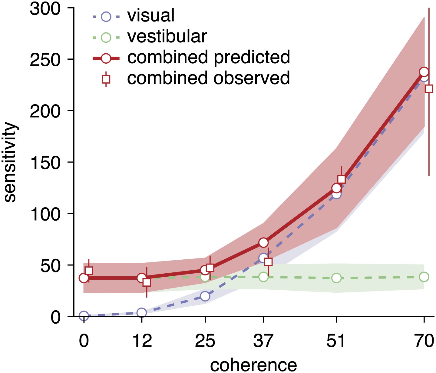
Predicted and observed sensitivity in the combined condition.
The sensitivity parameter measures how sensitive subjects are to a change of heading. The solid red line shows predicted sensitivity for the combined condition, as computed from the sensitivities of the unimodal conditions (dashed lines). The combined sensitivity measured by fitting the model to each coherence separately (red squares) does not differ significantly from the optimal prediction, providing strong support to the hypothesis that subjects accumulate evidence near-optimally across time and cues. Data are averaged across datasets (except 0%, 12%, 51% coherence: only datasets B2, D2, F2), with shaded areas and error bars showing the 95% CIs.
Figure 7 with 2 supplements
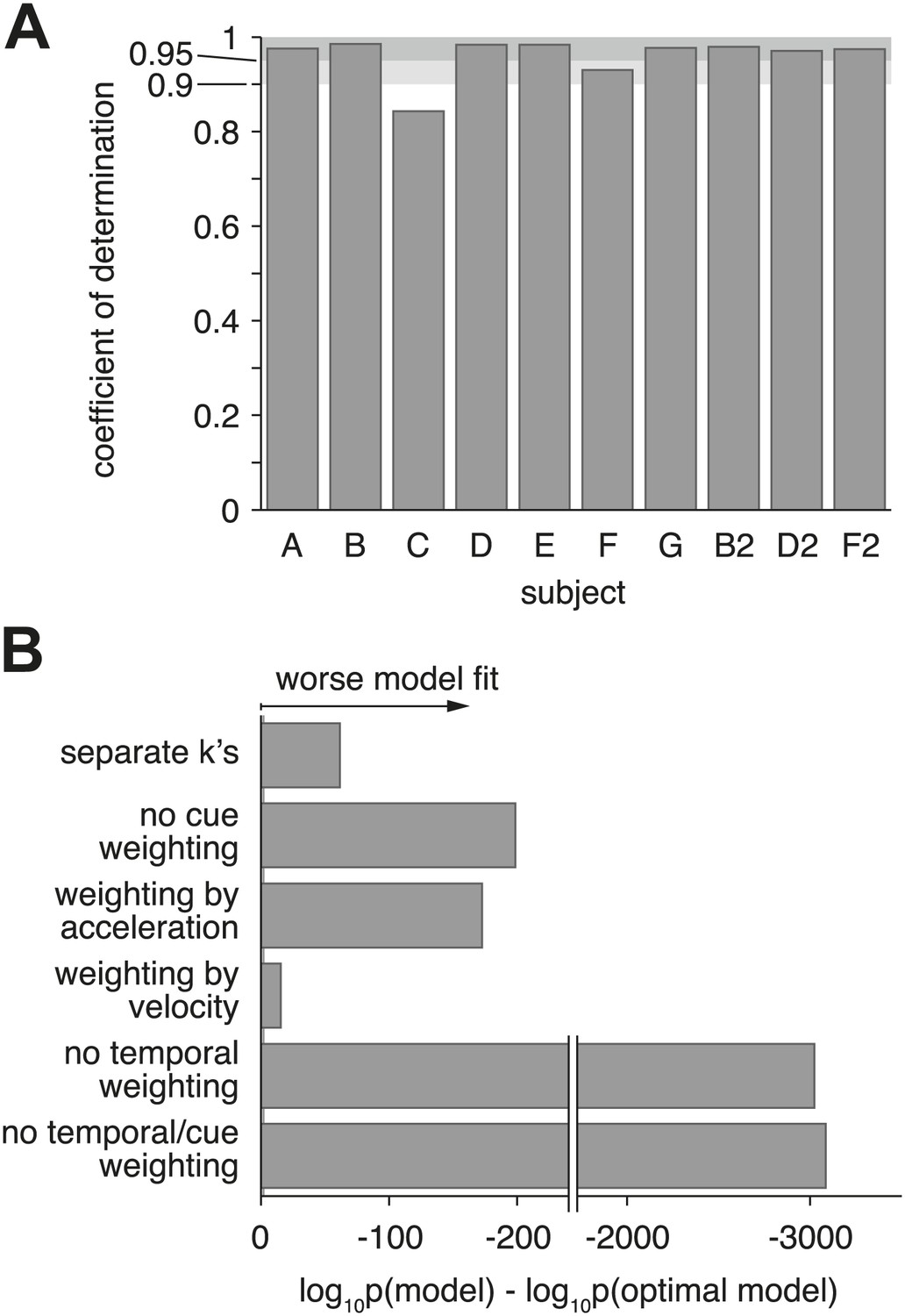
Model goodness-of-fit and comparison to alternative models.
(A) Coefficient of determination (adjusted R2) of the model fit for each of the ten datasets. (B) Bayes factor of alternative models compared to the optimal model. The abscissa shows the base-10 logarithm of the Bayes factor of the alterative models vs the optimal model (negative values mean that the optimal model out-performs the alternative model). The gray vertical line close to the origin (at a value of −2 on the abscissa) marks the point at which the optimal model is 100 times more likely than each alternative, at which point the difference is considered ‘decisive’ (Jeffreys, 1998). Only the ‘separate k's‘ model has more parameters than the optimal model, but the Bayes factor indicates that the slight increase in goodness-of-fit does not justify the increased degrees of freedom. The ‘no cue weighting’ model assumes that visual and vestibular cues are weighted equally, independent of their sensitivities. The ‘weighting by acceleration’ and ‘weighting by velocity’ models assume that the momentary evidence of both cues is weighted by the acceleration and velocity profile of the stimulus, respectively. The ‘no temporal weighting’ model assumes that the evidence is not weighted over time according to its sensitivity. The ‘no cue/temporal weighting’ model lacks both weighting of cues by sensitivity and weighting by temporal profile. All of the tested alternative models explain the data decisively worse than the optimal model. Figure 7—figure supplement 1 shows how individual subjects contribute to this model comparison, and the results of a more conservative Bayesian random-effects model comparison that supports same conclusion. Figure 7—figure supplement 2 compares the proposed model to ones with alternative parameterizations.
Figure 7—figure supplement 1

Model comparison per subject, and random-effects model comparison.
(A) Shows the contribution of each subject to the model comparison shown in Figure 7B. As in Figure 7B, the grey line shows the threshold above which the alternative models provide a decisively worse (if negative) or better (if positive) model fit. As can be seen, the model comparison is mostly consistent across subjects, except for models that weight both modalities either by acceleration or velocity only. Even in these cases, pooling across subjects leads to a decisively worse fit of the alternative model when compared to the optimal model (Figure 7). (B) and (C) Show the results of a random-effects Bayesian model comparison (Stephan et al., 2009). This model comparison infers the probability of each model to have generated the behavior observed for each subject, and is less sensitive to model fit outliers than the fixed-effects comparison shown in Figure 7B (e.g., a single subject might strongly support an otherwise unsupported model, which could skew the overall comparison). (B) Shows the inferred distribution over all compared models, and supports the optimal model with exceedance probability p≈0.664 (probability that the optimal model is more likely that any other model). This random-effects comparison causes models with very similar predictions to share some probability mass—in our case the optimal model and the model assuming evidence weighting by the velocity time-course. In (C) we perform the same comparison without the ‘weighting by velocity’ model, in which case the exceedance probability supporting the optimal model rises to p≈0.953.
Figure 7—figure supplement 2
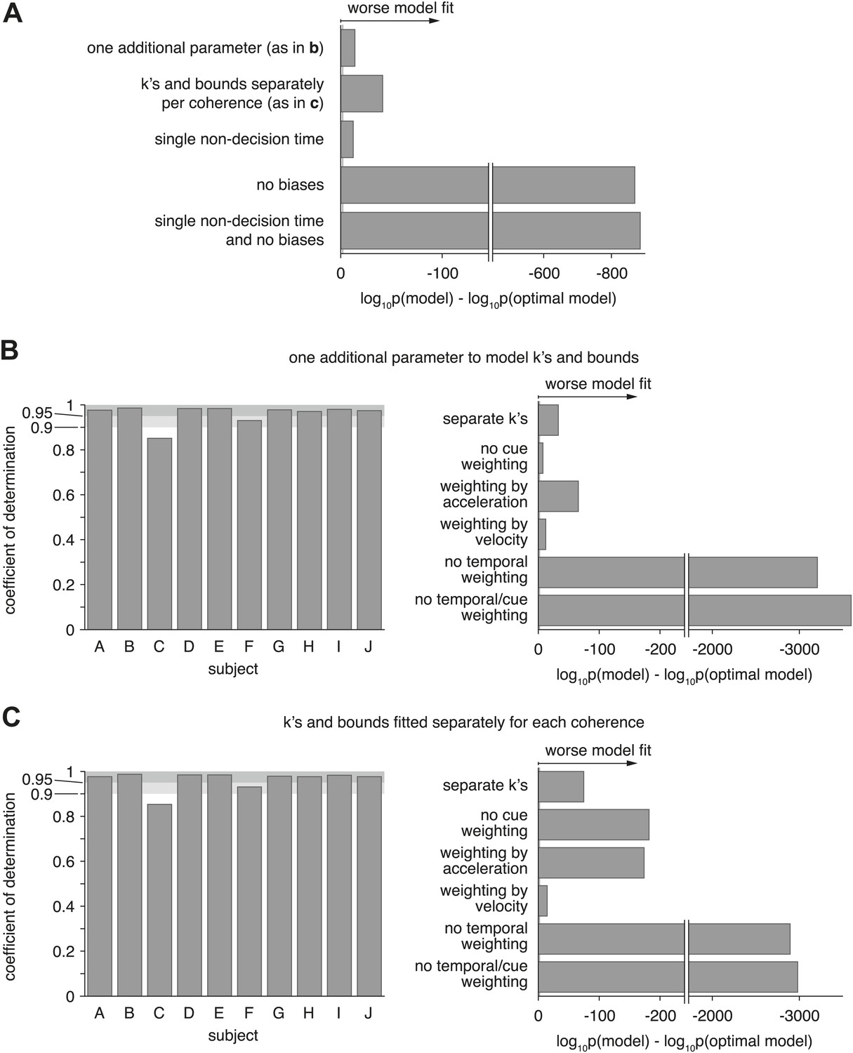
Model comparison for models with alternative parameterization.
(A) Compares the optimal model as described in the main text to various alternative models. The first model changes how drifts and bounds relate to coherence (see Supplementary file 1), and introduces one additional parameter. The second model fits drifts and bounds separately for all coherences. The other models either use a single non-decision time (instead of one or each modality), no heading biases, or a combination of both. The figure shows the Bayes factor, illustrating that in all cases the alternative models are decisively worse (grey line close to origin indicating threshold) than the original model. (B and C) Show the overall model goodness-of-fit (left panels) of two model that used an alternative parameterization of how drifts and bounds depend on coherence (see (A)). Furthermore, it compares these models, which still perform optimal evidence accumulation across both time and cues, to sub-optimal models (right panels) that do not (except ‘separate k's’, which is potentially optimal). These figures are analogous to Figure 7 and show that neither change of parameterization qualitatively changes our conclusions.
Additional files
-
Supplementary file 1
Detailed model derivation and description.
- https://doi.org/10.7554/eLife.03005.015
-
Supplementary file 2
Outcome of additional statistical hypothesis tests.
- https://doi.org/10.7554/eLife.03005.016
Download links
A two-part list of links to download the article, or parts of the article, in various formats.
Downloads (link to download the article as PDF)
Open citations (links to open the citations from this article in various online reference manager services)
Cite this article (links to download the citations from this article in formats compatible with various reference manager tools)
Optimal multisensory decision-making in a reaction-time task
eLife 3:e03005.
https://doi.org/10.7554/eLife.03005


