Mechanical design principles of a mitotic spindle
- European Molecular Biology Laboratory, Germany
- University of Oxford, United Kingdom
- Institut Génétique Biologie Moléculaire Cellulaire, France
Figures
Figure 1 with 1 supplement
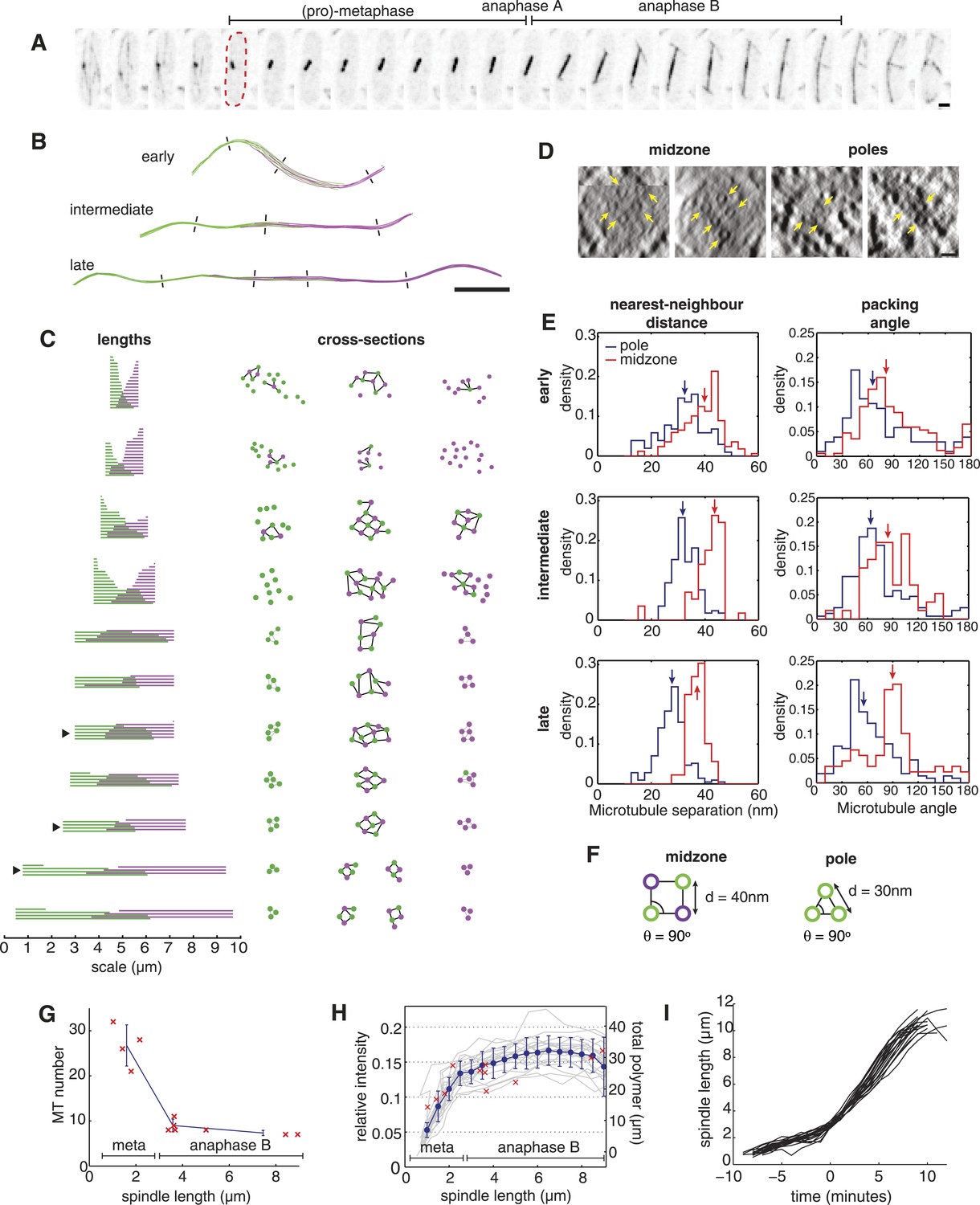
The Architecture and Dynamics of the Fission Yeast Spindle.
(A) Fission yeast cell expressing GFP-labelled tubulin. The dashed red line shows cell outline at mitotic entry. Interval between frames = 1 min, scale bar = 0.5 μm. (B) ET reconstructions of three anaphase B spindles. Microtubules are coloured according to the pole from which they originate. Dashes represent the approximate locations of the cross-sections shown in C. (C) Longitudinal and transverse spindle architecture. Diagrams on the left show the contour length and number of microtubules within each spindle. Black arrowheads mark the three anaphase B spindles depicted in B. Circle-and-stick diagrams on the right represent cross-sections near to the poles and midzone of each spindle. Microtubule radii are drawn to scale. Black lines are drawn between neighbouring anti-parallel microtubules. (D) Raw electron tomographic images of second-longest anaphase B spindle shown in C. Microtubules are marked by yellow arrows. Scale bar = 25 nm. (E) Histograms of nearest-neighbour microtubule distances and packing angles for the three spindles shown in panel B. Blue lines represent histograms for the polar regions of the spindle and red lines the midzone. Coloured arrows mark the median of each distribution. The midzone is defined as the region of microtubule overlap that contains at least two microtubules from each pole. Kolmogorov–Smirnov tests were used to determine the probability that distributions for the polar and midzone regions were drawn from the same parent. All of the comparisons, shown here, have a p-value <10−4. (F) Schematic representation of microtubule angle and distance distributions at the poles and midzone of the spindle. (G) Number of spindle microtubules with respect to pole-to-pole spindle length Ls. The blue error bars summarise results for spindles divided into metaphase (Ls < 2.5 μm), early anaphase B (2.5 < Ls < 4 μm), and late anaphase B (Ls > 4 μm) stages. (H) Estimates of the ratio of fluorescent tubulin incorporated into the spindle for twenty mitotic cells (grey curves) with mean and standard deviations shown in blue. The red crosses indicate the total length of microtubules polymerised within each ET spindle. (I) Elongation profile for twenty wild-type spindles obtained from automatic tracking of SPBs. The traces are aligned temporally by defining time-zero as the frame at which spindles first reach a length of 3 μm.
Figure 1—figure supplement 1
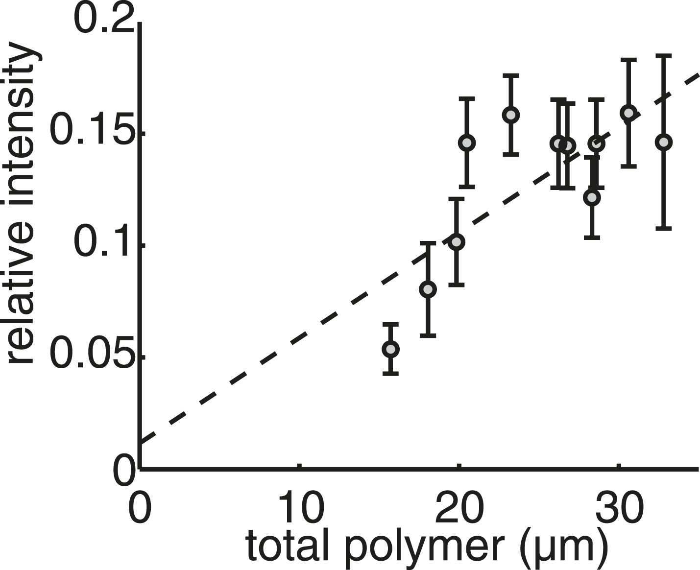
Live-cell imaging confirms that the mass of tubulin polymerised in the spindle is conserved throughout anaphase B.
Linear calibration curve for relating polymer mass to spindle intensity. Coefficient of determination R2 = 0.40.
Figure 2
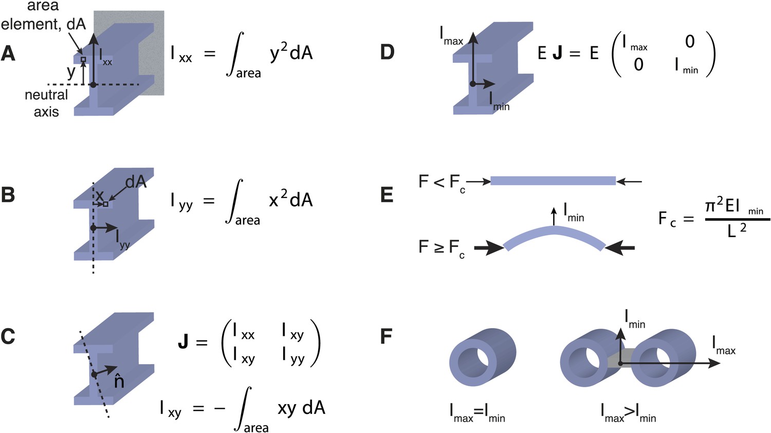
Effects of Transverse Organisation on the Critical Force of Prismatic Beams.
(A) The Ι-beam is a structural element that is commonly used in civil engineering. If the beam is clamped in a horizontal position at the end furthest from view (grey rectangle), and a transverse force is applied at the other end (in this case upwards), then the beam's resistance is defined by the scalar transverse stiffness, EIxx, which is the product of the Young's modulus, E, and the area moment of inertia, Ixx. The area moment of inertia can be computed by dividing the cross-section into area elements, dA, and multiplying each area by the square of their distance, y, from the neutral axis (dotted line). A sum or integration of this quantity can then be used to compute the area moment of inertia, Ixx. The neutral axis is perpendicular to the applied force and passes through the centre-of-mass of the beam's cross-section. Intuitively, an increased stiffness can be achieved by placing the beam's material as far from the neutral axis as possible. This property is the rationale behind the design of the I-beam, which typically bears loads in the direction given by Ixx. (B) A similar calculation to A can be used to calculate the beam's stiffness in an orthogonal direction. It is usually the case that Ixx > Iyy for Ι-beam designs. (C) The generalised response of a beam to forces in an arbitrary direction, denoted by the unit vector n, can be represented by the area moment of inertia tensor, J, with entries Ixx, Iyy, Ixy. The tensor, J, is a matrix quantity that relates the direction of the applied force to the beam's deflection (Landau et al., 1986). For a general tensor matrix, there exist two orthogonal vectors (known as eigenvectors) that represent the directions of the beam's maximal and minimal stiffness. (D) The eigenvectors or principal axes of the Ι-beam point along the x and y-axes. (E) Under purely compressive forces a prismatic beam with length, L, will buckle in the direction of the most compliant principal axis, which defines the critical force, Fc, for beams of this type. (F) Beams with a mechanically isotropic transverse organisation, such as microtubules, have a scalar stiffness tensor (Imin = Imax) and degenerate principal axes. The ratio Imax/Imin ≥ 1 can be used to quantify the beam's degree of anisotropy. The ratio is one for mechanically isotropic structures such as a single microtubule or a bundle of 4 microtubules arranged in a 2 × 2 square motif.
Figure 3 with 1 supplement
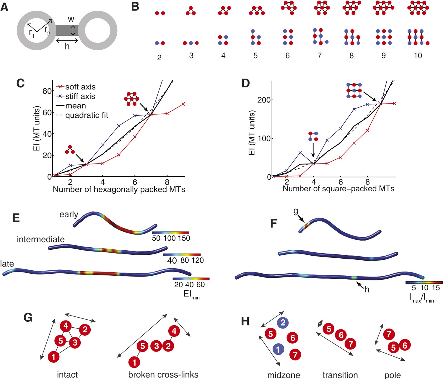
The Cross-Sectional Microtubule Organisation Enhances the Spindle's Transverse Stiffness.
(A) Schematic representation of a pair of bundled microtubules. Microtubules are modelled as hollow cylinders that are linked by rectangular support elements with identical material properties. In all moment of inertia calculations we used r1 = 7.5 nm and r2 = 12.5 nm. (B) Transverse organisation of idealised hexagonal and square-packed arrays of microtubules as additional fibres are added. (C, D) Eigenvalues of the stiffness tensor for idealised hexagonal and square-packed microtubule arrays. Results are shown for centre-to-centre separations (equal to h+2 r2) that match those obtained from ET reconstructions. These are 30 nm and 40 nm for hexagonal (polar) and square (midzone) arrays, respectively. The blue and red curves show the small and large eigenvalues of the stiffness tensor. Black arrows represent microtubule organisations with degenerate eigenvalues and isotropic stiffness. The solid black curves show the mean of the large and small eigenvalues, and the dashed black curves a quadratic fit to the mean stiffness. The y-axis (labelled as MT units) shows the stiffness of the bundle divided by the stiffness of one microtubule. (E) Minimal transverse stiffness, EImin, for three anaphase B spindles with identical units to C, D. (F) Stiffness anisotropy ratio, Imax/Imin, color-coded over the ET spindle reconstructions. Arrows mark the positions of the regions shown in G and H. (G) An apparent loss of cross-linker integrity at the pole of the spindle is a cause of stiffness anisotropy. Microtubules are drawn to scale, and are numbered consistently between slices. Arrows show the approximate extent of the bundle in two orthogonal directions. The two sections are separated by a distance of 240 nm along the spindle axis. (H) Transverse sections showing stiffness anisotropy at the transition from the square-packed crystalline phase to hexagonal phase. Each slice is separated by an axial distance of 200 nm.
Figure 3—figure supplement 1
Transverse Stiffness of Cross-linked Microtubule Bundles.
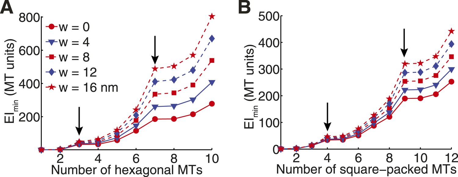
(A) Minimal transverse stiffness of a cross-linked hexagonal array of microtubules. Curves reflect the small eigenvalue of the stiffness tensor for cross-linkers of increasing width. Other constants are identical to those described in panel D from the main text. Arrows mark the position of hexagonal structural motifs. (B) Minimal transverse stiffness of square-packed bundles of microtubules with variable cross-link width.
Figure 4 with 1 supplement
Computational Reconstructions of the Spindle can be used to Estimate its Effective Stiffness.
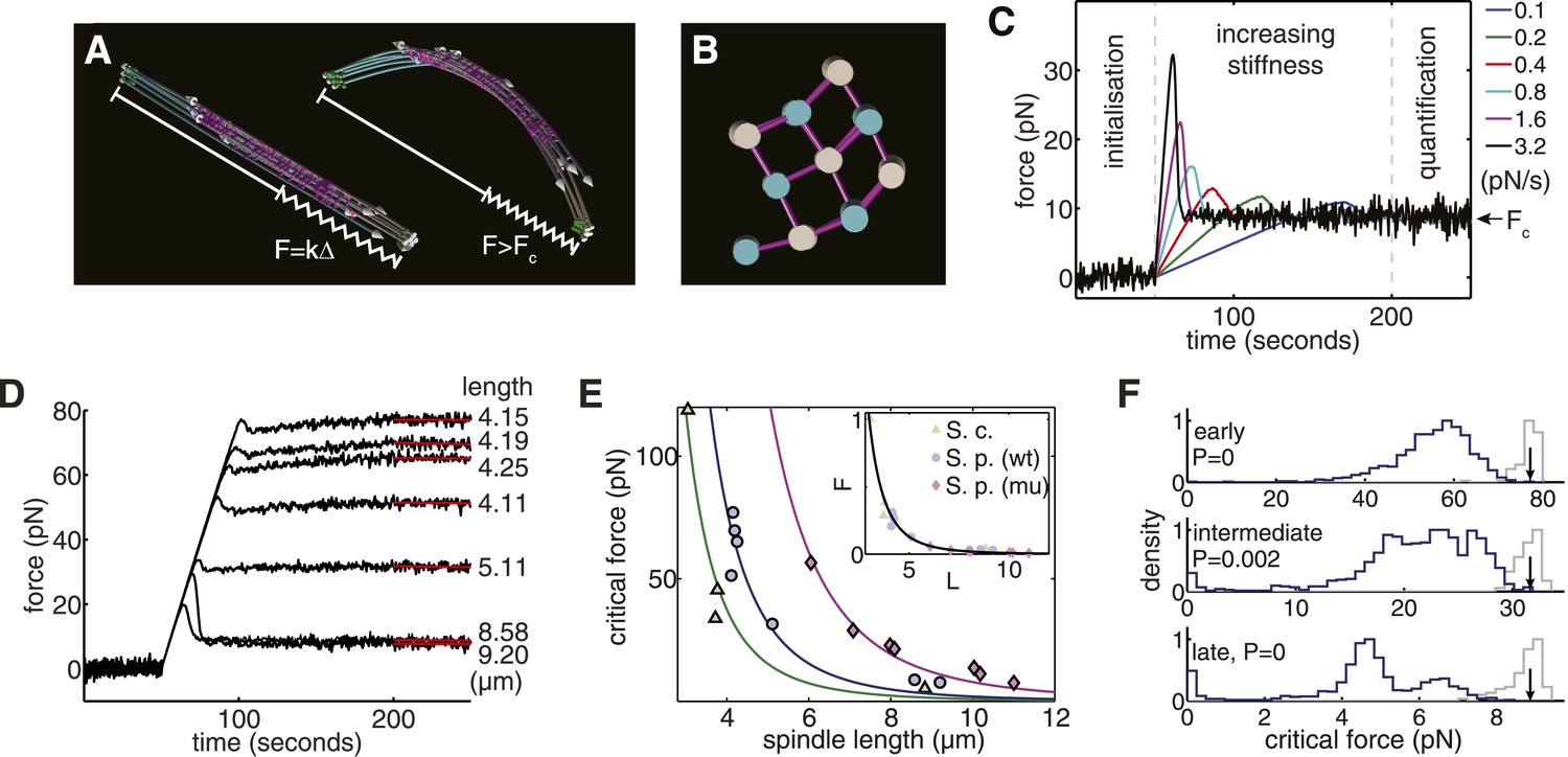
(A) Computational reconstruction of an early anaphase B spindle before and after the critical force is exceeded. The spindles are subjected to compression by attaching a spring between the spindle poles. The elastic constant is then increased to probe the spindle's response to force. (B) Stochastic initialisation conditions can reproduce the 3 × 3 organisation at the midzone of a spindle in early anaphase B. Microtubules are depicted with a diameter of 25 nm. (C) Model response of the longest fission yeast spindle to forces that increase at different rates. The SPBs are held at the spindles' contour separation for the first 50 s of the simulation, when cross-linkers are allowed to form attachments between the two halves of the bipolar spindle. At t = 50 s, the elastic constant of the spring connecting the two SPBs is then set to zero and its resting length reduced to Δ = 1 μm less than the SPB's resting separation. The elastic constant is then increased linearly over the subsequent 150 s of the simulation to exert progressively larger force on the spindle. Each colour, represented in the legend, denotes a different force increase in units of pNs−1. The spindles bear the increasing compressive loads until a threshold is reached and the force decays before plateauing at the equilibrium (critical) force, Fc. In the final 50 s of the simulation (marked quantification), the spring constant of the elastic element connecting the SPBs is maintained at its maximal value, and the critical force quantified by averaging the force-response profile. (D) Response of fission yeast spindle models to compressive forces. The contour length of each spindle is noted in the right-hand column. Curves show the median critical force from N = 100 stochastic simulations. (E) Dependence of critical force on spindle length for models of w.t. S. pombe, cdc25.22 S. pombe and Saccharomyces cerevisiae anaphase B spindles. Each point indicates the median critical force calculated from N = 100 simulations. Curves show Fc = ALs−4 fits to the simulation results, where the only fit parameter is the pre-factor, A. Inset shows normalised force Fc/A = Ls−4 for all spindle types. This rescaling highlights the universality of the relationship between spindle length and critical force. (F) Comparison of the critical force of fission yeast spindles (grey histograms, N = 100) with a null statistical model (blue histograms, N = 103). p-values refer to the probability that a random spindle has a critical force greater than the median wild-type spindle.
Figure 4—figure supplement 1
Compressive Strength and Optimality of Yeast Spindles.
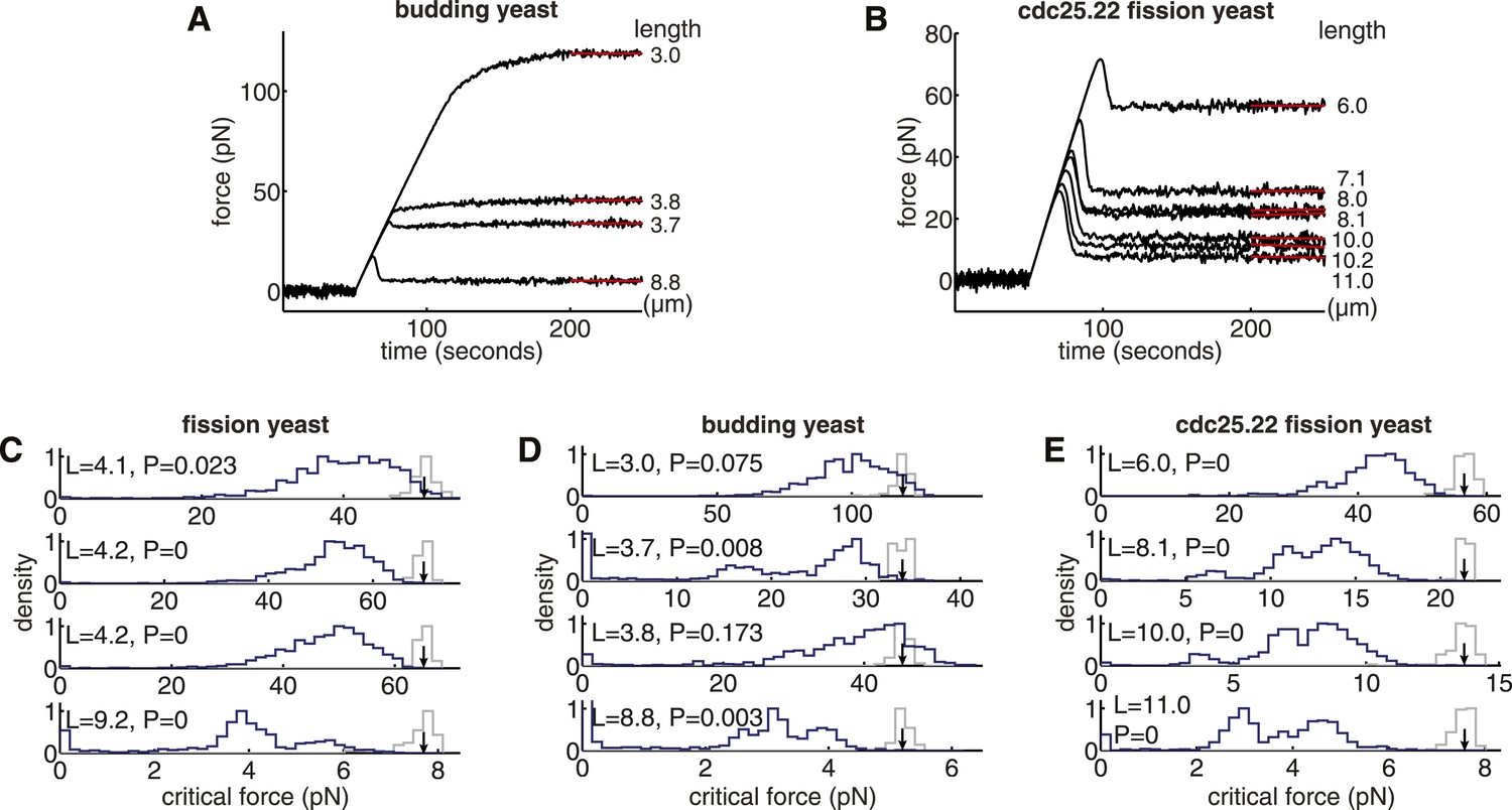
(A, B) Response of budding yeast and cdc25.22 spindle models to compressive forces. The pole-to-pole length of each spindle is noted in column to the right of each plot. (C–E) Comparisons of the critical force of anaphase B spindles in wild-type fission yeast, budding yeast and cdc25.22 fission yeast cells with a null model of each spindle architecture. The spindle length is shown in the top-left corner of each plot. The blue histograms show the critical force of 1000 realisations of the null model, in which the lengths and number of microtubules are sampled randomly. The grey histograms show the critical force estimated from N = 200 simulations of the wild-type spindle architecture with the medians represented by black arrows. p-values refer to the probability that a random spindle has a critical force greater than that of the median wild-type spindle.
Figure 5 with 1 supplement
Fission Yeast Spindles Scale Microtubule Lengths and Number for Maximal Overlap at the Spindle Midzone.
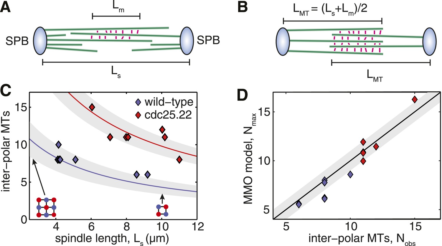
(A) Schematic representation of a fission yeast spindle of length Ls. Green lines represent microtubules and magenta lines anti-parallel cross-linkers, which bind to the midzone region of width Lm. Blue shaded ellipses represent the spindle pole bodies (SPBs). (B) Maximal anti-parallel bundling of microtubules at the spindle midzone is achieved if microtubules have a monodisperse length LMT = (Ls + Lm)/2. (C) Number of interpolar microtubules in wild-type and cdc25.22 mutant fission yeast cells with respect to spindle length (blue and red diamonds, respectively). Trend lines show theoretical calculation of microtubule number in MMO spindle architecture based on the spindle length, Ls, and average total polymer, LT. For wild-type cells LT = 27.1 S.D. 4.2 μm (blue curve with standard deviation represented by grey shaded area) whilst for cdc25.22 cells LT = 61.2 S.D. 7.8 μm (red curve). (D) Comparison of interpolar microtubule number with predictions of the MMO model. The black line shows trend for exact agreement with grey bars representing 1 microtubule deviation.
Figure 5—figure supplement 1
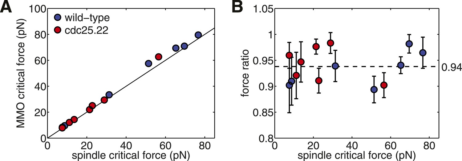
Critical force of Wild-type and Cdc25.22 Mutant Fission Yeast Cells.
(A) Critical force for simulations of wild-type spindles compared with MMO spindles with the same quantity of polymer mass. Points reflect the median from 200 stochastic simulations of each condition. (B) Ratio of median critical force of wild-type spindle architectures compared with the distribution of critical forces for MMO spindles. Error bars represent a single standard deviation.
Figure 6
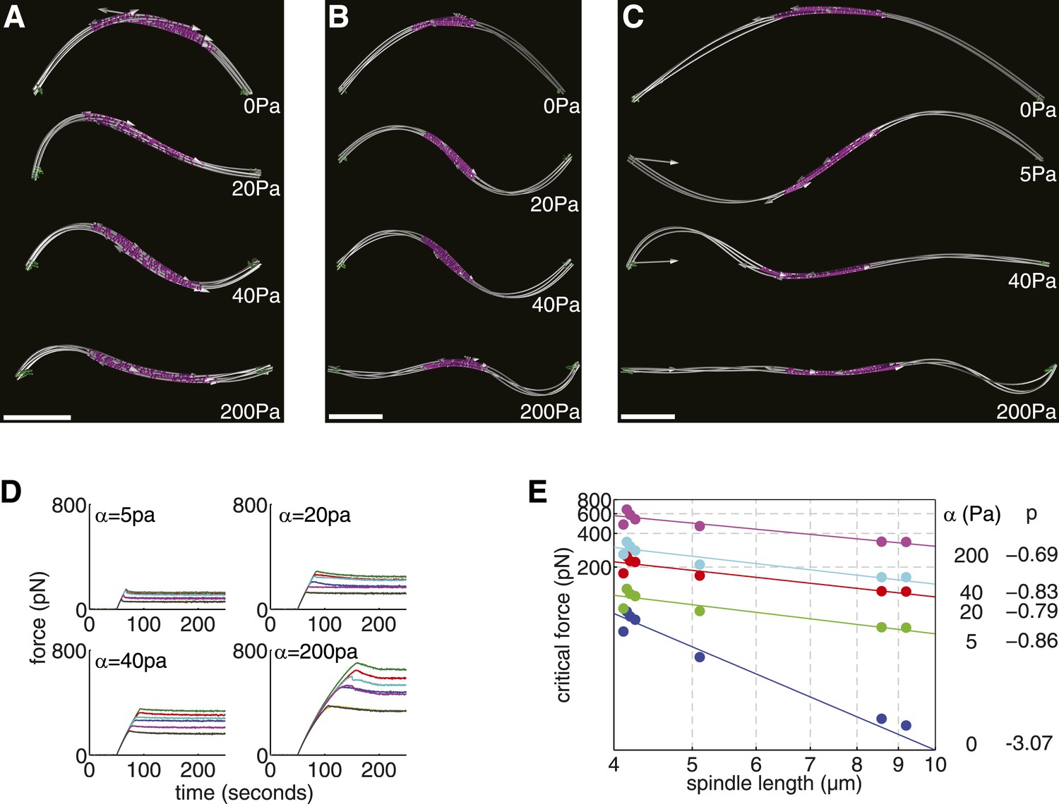
Elastic Reinforcement Enhances the Compressive Loads that can be Borne by the Spindle.
(A–C) Equilibrium shapes adopted by exemplary anaphase B spindles after the critical force is exceeded. The degree of lateral reinforcement, α, is shown alongside each simulation. Scale bars = 1 μm. (D) Force-response of reconstructed anaphase B spindles (median critical force calculated from the results of 50 stochastic simulations). (E) Relationship between the critical force of laterally reinforced spindles and their length. Lines reflect power law fits Fc = ALp, with exponent, p, shown to the right of each curve.
Figure 7
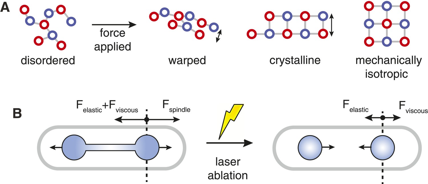
Spindle Resistance To Compressive Forces.
(A) Applying compressive force to a sparsely connected microtubule bundle leads to warping. This increases bundle anisotropy and leads to a reduction in the critical force. In a crystalline microtubule array, microtubules can associate with a larger number of neighbouring microtubules. This constrains microtubule movement and increases the transverse stiffness. Arranging the crystal unit cells with rotational symmetry leads to architectures with an isotropic resistance to bending forces and an increased minimal transverse stiffness. (B) In late anaphase B, the forces driving spindle elongation are balanced by the viscoelastic response of the cytoplasm and an elastic force. After ablation of the spindle midzone, this elastic force is opposed by the viscous drag.
Videos
Video 1
Spindle formation and elongation in fission yeast.
Frames are shown at intervals of 1 min. The green channel shows maximum intensity projections of cells expressing GFP-tubulin (SV40:GFP-Atb2), with the magenta channel showing SPBs labelled with Cut12-tdTomato. The cut12-tdTomato images were processed using a deconvolution algorithm.
Video 2
Summed intensity projections of GFP-tubulin in mitotic fission yeast cell augmented with tracking and segmentation results.
The cell outline is shown in magenta. The magenta circles represent tracking of the SPBs from the cut12-tdTomato channel (not shown). These are used to define the green box, which is used to compute spindle intensity. Tracking of the spindle intensity is ceased after the spindle elongates beyond 9 μm. At later stages of elongation more pronounced buckling of the spindle is observed, and microtubules begin to be nucleated in the vicinity of the cytokinetic ring.
Video 3
Electron Tomogram (ET) reconstruction of short anaphase B spindle.
from Figure 1B, top. Scale bar = 0.5 μm.
Video 4
Electron Tomogram (ET) reconstruction of intermediate length anaphase B spindle.
from Figure 1B, middle. Scale bar = 0.5 μm.
Video 5
Electron Tomogram (ET) reconstruction of long anaphase B spindle.
from Figure 1B, bottom. Scale bar = 0.5 μm.
Video 6
Simulation of Spindle Subjected to Compressive Forces.
In the first 50 s of the simulation, the force exerted on the poles of the spindle is zero, and cross-linkers are allowed to bind and unbind from the microtubule lattice to form attachments between the two halves of the bipolar spindle. After 50 s the force on the spindle increases linearly until buckling is induced (Figure 4C,D).
Video 7
Simulation of Short, Intermediate and Long Example Spindles Subjected to Compressive Forces with Differing Degrees of Lateral Reinforcement.
Scale is set by the size of the enclosing cell, which measures 11 μm in length between the opposite cell tips. From the image at the top downwards, the spindles are subjected to increasing confinement with α = 0, 20, 40, 200 Pa, respectively for the short and intermediate length spindles. For the longest spindle, α = 0, 5, 40, 200 Pa.
Video 8
Simulation of Short, Intermediate and Long Example Spindles Subjected to Compressive Forces with Differing Degrees of Lateral Reinforcement.
Scale is set by the size of the enclosing cell, which measures 11 μm in length between the opposite cell tips. From the image at the top downwards, the spindles are subjected to increasing confinement with α = 0, 20, 40, 200 Pa, respectively for the short and intermediate length spindles. For the longest spindle, α = 0, 5, 40, 200 Pa.
Video 9
Simulation of Short, Intermediate and Long Example Spindles Subjected to Compressive Forces with Differing Degrees of Lateral Reinforcement.
Scale is set by the size of the enclosing cell, which measures 11 μm in length between the opposite cell tips. From the image at the top downwards, the spindles are subjected to increasing confinement with α = 0, 20, 40, 200 Pa, respectively for the short and intermediate length spindles. For the longest spindle, α = 0, 5, 40, 200 Pa.
Tables
Table 1
Measurements for calculation of critical and absolute tubulin concentration in fission yeast
| Cell dimensions | ||
|---|---|---|
| Radius | Rc = 1.6 ± 0.1 μm | Maximal cell diameter/2 (Foethke et al., 2009) |
| Length | Lc = 14.3 ± 0.9 μm | Distance between cell tips at mitotic entry (Martin and Berthelot-Grosjean, 2009; Moseley et al., 2009) |
| Volume | Vc = 2πRc3.(Lc/2Rc−1/3) Vc = 106.4 ± 13.4 μm3 | Assumes cell is sphero-cylindrical |
| Spindle properties | ||
| Steady-state polymer | 27.1 ± 4.2 μm | Sum of all the microtubule's length. This study |
| α/β-tubulin heterodimers | (4.4 ± 0.6) × 104 dimers | Each MT has 13-protofilaments with a length of 8 nm (Howard, 2001) |
| Relative intensity | 0.16 ± 0.02 | Mean fluorescent intensity ratio of spindles longer than 4 μm |
| Tubulin dimer concentration | ||
| Abundance | (20.0 ± 4.0) × 104 | Number of dimers in the cell |
| Free pool | 3.61 ± 0.68 μM | Corresponds to the critical concentration of MT assembly |
| Polymerized pool | 0.68 ± 0.13 μM | |
| Total concentration | 4.30 ± 0.81 μM | |
Table 2
Physical and numerical constants for simulations of spindle stiffness
| Description | Value | Notes |
|---|---|---|
| Global | ||
| kBT | 0.0042 pN.μm | Thermal energy at T = 27°C |
| Viscosity | 1 pN pN.s.μm−2 | Viscosity of fission yeast cytoplasm (Tolić-Nørrelykke, Munteanu, et al., 2004a) |
| Time step | 0.001 s | Simulations with smaller time-steps produce similar results |
| Microtubules | ||
| Segmentation | 0.1 μm | |
| Flexural rigidity | 20 pN.μm2 | This is EIMT (Gittes et al., 1993) |
| Steric radius | 30 nm | Microtubule outer radius + Debye length |
| Steric stiffness | 200 pN.μm−1 | per microtubule segment |
| Midzone width | 2.5 μm | (Loïodice et al., 2005; Yamashita et al., 2005) |
| Spindle Pole Bodies | ||
| Radius | 60 nm | Observed from ET |
| Depth | 100 nm | Observed from ET |
| Stiffness 1 | 1000 pN.μm−1 | Appropriate for (Khodjakov et al., 2004) (Tolić-Nørrelykke, Sacconi, et al., 2004b) (Toya et al., 2007) |
| Stiffness 2 | 20 pN.μm−1 | Appropriate for (Kalinina et al., 2013) |
| Cross-linkers | ||
| Number | 300 | Less than abundance of ase1p (∼900 dimers/cell) and klp9p (∼1300 dimers/cell) (Marguerat et al., 2012). Larger numbers do not alter simulation results |
| Bridging length | 50 nm | Approximate centre-to-centre distance of microtubules bundled by Map65 proteins (Subramanian et al., 2010). |
| Link stiffness | 1000 pN.μm−1 | Force is Hookean with a non-zero resting length (Howard, 2001) |
Table 3
Estimates of forces resisting spindle elongation
| Description | Variable | Value | Notes |
|---|---|---|---|
| Cell radius | rcell | 1.6 μm | (Foethke et al., 2009) |
| Daughter nuclei radius | rnucleus | 0.8–1.0 μm | This study (ET estimate)−21/3 × radius of interphase nucleus (Foethke et al., 2009) |
| Cytoplasmic viscosity | ηcell | 1 pN.s.μm−2 | (Tolić-Nørrelykke, Munteanu, et al., 2004a) |
| Spindle pole separation speed | vs | 0.9 μm.min−1 | This study |
| Drag coefficient | γ | 25-110 pN.μm−1.s | See ‘Materials and methods’ |
| Relaxation time | τ = γ/k | 9.7 s | Exponential fit to collapse of long spindle (Khodjakov et al., 2004), Figure 7B |
| Equilibrium position | x0 | 1.4 μm | Second fit parameter |
| Drag force | Fv = γ.vs/2 | 0.2–0.8 pN | |
| Elastic force | Fe = x0.γ/ τ | 3–16 pN | This force is dramatically decreased after the nucleus adopts a dumbbell configuration |
| Total force | Fe + Fv | 4–17 pN |
Additional files
-
Source Code 1
Compressed plain text files containing raw data, scripts and analysis code. The directory ‘EM_analysis’ includes microtubule coordinates for eleven fission yeast spindles that were reconstructed using ET, in addition to MATLAB (The MathWorks inc.) programs for performing geometric analysis on the spindles' architecture. Scripts used to perform analyses of live-cell fluorescent imaging of fission yeast mitosis are included in the directory, ‘LM_analysis’. The directory, ‘simulation_configs’ contains Cytosim configuration files for simulations of yeast spindles buckling under compressive force.
- https://doi.org/10.7554/eLife.03398.026
Download links
A two-part list of links to download the article, or parts of the article, in various formats.
Downloads (link to download the article as PDF)
Open citations (links to open the citations from this article in various online reference manager services)
Cite this article (links to download the citations from this article in formats compatible with various reference manager tools)
Mechanical design principles of a mitotic spindle
eLife 3:e03398.
https://doi.org/10.7554/eLife.03398


