Speech encoding by coupled cortical theta and gamma oscillations
- Ecole Normale Supérieure, France
- University of Geneva, Switzerland
- National Research University Higher School, Russia
Figures
Figure 1 with 1 supplement
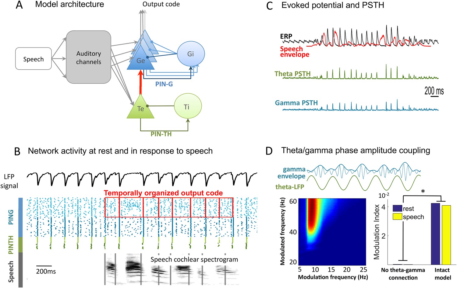
Network architecture and dynamics.
(A) Architecture of the full model. Te excitatory neurons (n = 10) and Ti inhibitory neurons (n = 10) form the PINTH loop generating theta oscillations. Ge excitatory neurons (n = 32) and Gi inhibitory neurons (n = 32) form the PING loop generating gamma oscillations. Te neurons receive non-specific projections from all auditory channels, while Ge units receive specific projection from a single auditory channel, preserving tonotopy in the Ge population. PING and PINTH loops are coupled through all-to-all projections from Te to Ge units. (B) Network activity at rest and during speech perception. Raster plot of spikes from representative Ti (dark green), Te (light green), Gi (dark blue), and Ge (light blue). Simulated LFP is shown on top and the auditory spectrogram of the input sentence "Ralph prepared red snapper with fresh lemon sauce for dinner" is shown below. Ge spikes relative to theta burst (red boxes) form the output of the network. Gamma synchrony is visible in Gi spikes. (C) Evoked potential (ERP) and Post-stimulus time histograms (PSTH) of Te and Ge population from 50 simulations of the same sentence: ERP (i.e., simulated LFP averaged over simulations, black line), acoustic envelope of the sentence (red line, filtered at 20 Hz), PSTH for theta (green line) and gamma (blue line) neurons. Vertical bars show scale of 10 spikes for both PSTH. The theta network phase-locks to speech slow fluctuations and entrains the gamma network through the theta–gamma connection. (D) Theta/gamma phase-amplitude coupling in Ge spiking activity. Top panel: LFP gamma envelope follows LFP theta phase in single trials. Bottom-Left panel: LFP phase-amplitude coupling (measured by Modulation Index) for pairs of frequencies during rest, showing peak in theta–gamma pairs. Bottom-right panel: MI phase-amplitude coupling at the spiking level for the intact model and a control model with no theta–gamma connection (red arrow on A panel), during rest (blue bars) and speech presentation (brown bars).
Figure 1—figure supplement 1
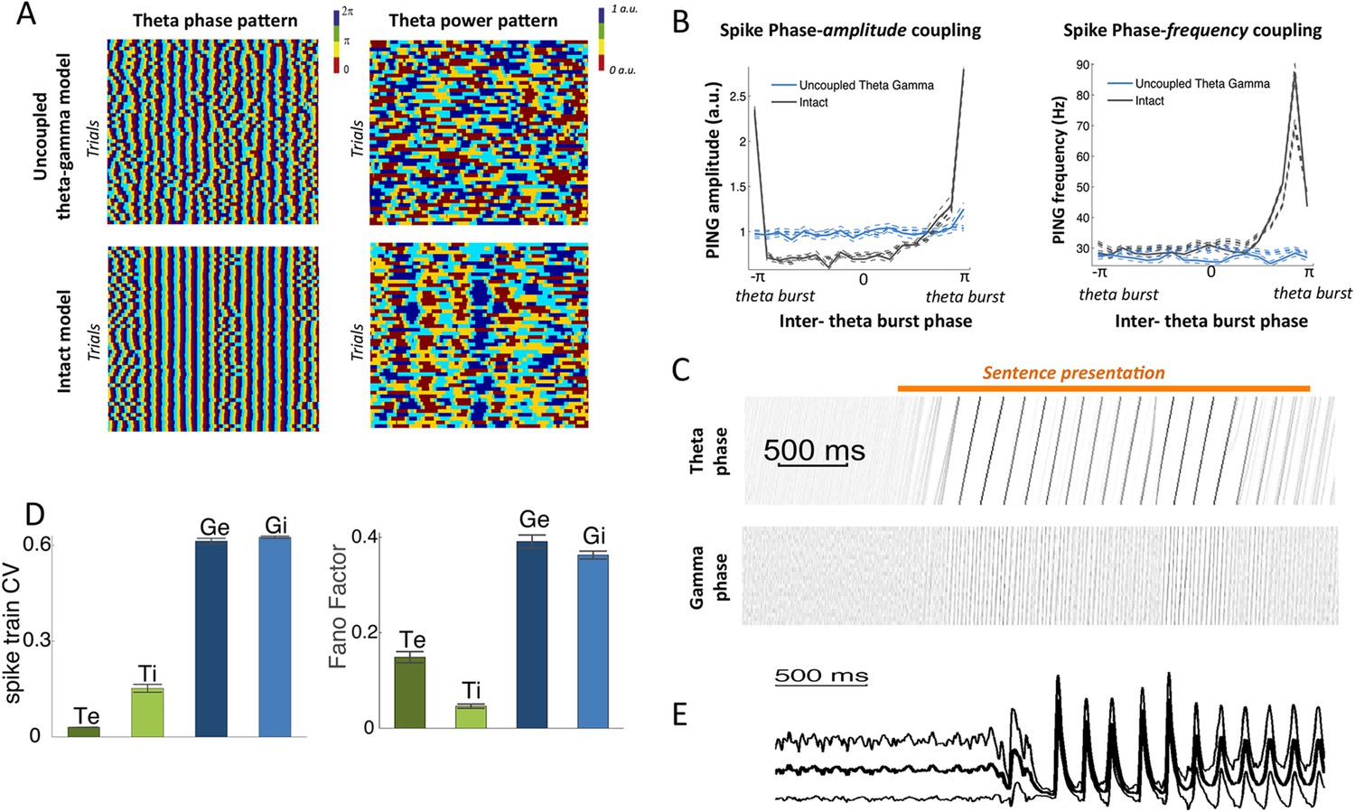
Spectral analysis.
(A) Theta phase pattern (left panels) and theta power pattern (right panels) for 50 presentations of the same sentence in the uncoupled theta–gamma control model (top panels) and intact panels (bottom panels). Phase/power is binned into 4 different bins and colour coded. Theta phase is much more reliably imprinted by speech stimulus than power. (B) (Left panel) Spike phase-amplitude coupling: mean value for PING amplitude (defined as the number of Gi neurons spiking within a gamma burst) as a function of PINTH phase (defined from interpolation between successive theta bursts). Intact model is shown in black while the uncoupled theta–gamma model is shown in blue. Data for rest (thick dashed lines) and during processing of speech (full thick lines) almost perfectly match. Thin dashed lines represent s.e.m. Spike PAC was very strong in the full model but quasi-absent when the theta–gamma connection was removed. (Right panel) Spontaneous spike phase-frequency coupling: mean value for PING frequency (defined from the duration between successive gamma bursts) as a function of PINTH phase. Same legend as left panel. Spike PFC is strong when and only when the theta–gamma connection is present (significant coupling p < 10−9 for both speech and rest). (C) Phase-locking of the theta and gamma oscillations to speech. Phase concentration of the filtered LFP theta (top panel) and gamma (bottom panel) signals through time for 200 presentations of the same sentence (same as Figure 1B,C). The horizontal orange bar indicates the presentation of the sentence. There is a rapid transition from uniform theta distribution before sentence onset to perfectly phase-locked theta. Phase-locking vanishes at the end of sentence presentation. (D) Spike pattern Coefficient of Variation (left) and spike count Fano factors (right) during speech presentation. Both measures were computed from the response of the network to 100 presentations of the same one-second speech segment. Bars and error bars represent mean and standard deviation over distinct neural populations. (E) LFP average (ERP) and standard deviation computed from the 100 repeats of presentation of the same sentence to the network. Note that the LFP variability is greatly reduced at speech onset, mainly due to phase-locking of theta and gamma oscillations.
Figure 2 with 1 supplement
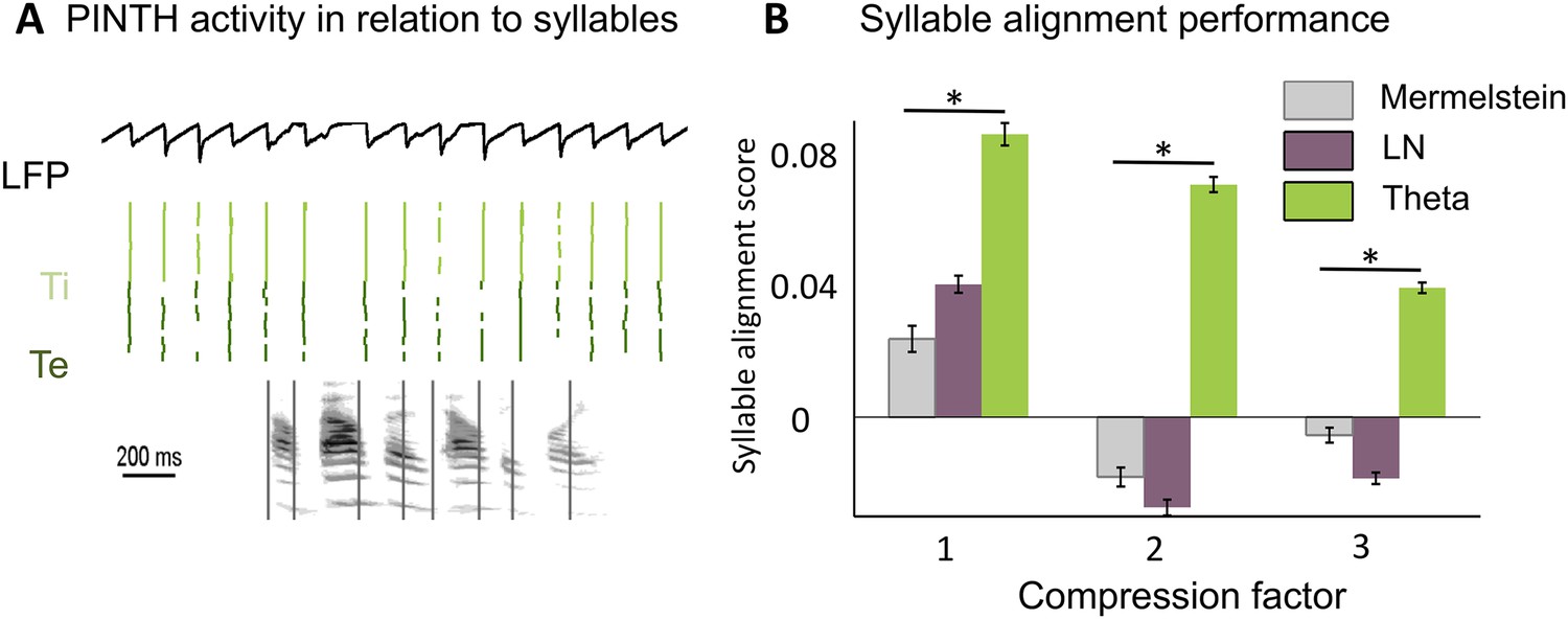
Theta entrainment by syllabic structure.
(A) Theta spikes align to syllable boundaries. Top graph shows the activity of the theta network at rest and in response to a sentence, including the LFP traces displaying strong theta oscillations, and raster plots for spikes in the Ti (light green) and Te (dark green) populations. Theta bursts align well to the syllable boundaries obtained from labelled data (vertical black lines shown on top of auditory spectrogram in graph below). (B) Performance of different algorithms in predicting syllable onsets: Syllable alignment score indexes how well theta bursts aligned onto syllable boundaries for each sentence in the corpus, and the score was averaged over the 3620 sentences in the test data set (error bars: standard error). Results compare Mermelstein algorithm (grey bar), linear-nonlinear predictor (LN, pink) and theta network (green), both for normal speed speech (compression factor 1) and compressed speech (compression factors 2 and 3). Performance was assessed on a different subsample of sentences than those used for parameter fitting.
Figure 2—figure supplement 1
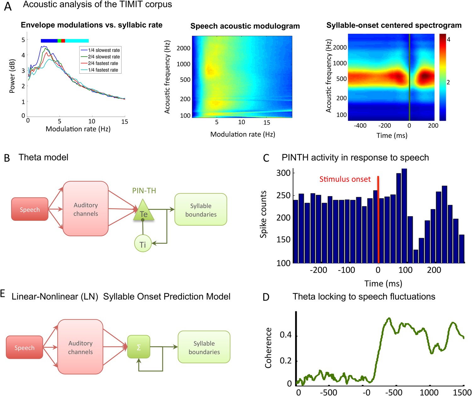
TIMIT corpus and models used for syllable boundary detection.
(A) Acoustic analysis of TIMIT corpus. Left panel: speech modulation frequency increases with syllabic rate. All 4620 sentences of the TIMIT corpus (Test data set) were sorted into quartiles according to syllabic rate (i.e., number of syllables per second). Speech envelope spectrum (with 1/f correction) was averaged over all sentences within each quartile, and the four averages are plotted. Colour bars on top of the graphs represent the syllabic rate range for all four quartiles, showing a correspondence between the modal frequency and the syllabic rate over the corpus. Middle panel: average channel spectrum. Spectrum was taken for each 128 auditory channels of the Chi and colleagues pre-cortical auditory model (Chi et al., 2005), averaged over all sentences in the corpus. All channels show a clear peak in the same 4–8 Hz range, showing that the theta modulation is very present in the input to auditory cortex. Right panel: syllable onset corresponds to a dip in spectrogram. Average of auditory spectrogram channels of sentences phase-locked to syllable onsets. t = 0 (green line) corresponds to syllable onset. Red colours correspond to high value, blue colours to low values. Dip at syllable onset is particularly pronounced over medium frequencies corresponding to formants. Auditory channels were averaged over all syllable onsets over the entire corpus (4620 sentences). This plot shows the connection between syllable boundaries and fluctuations of auditory channels that the auditory cortex may take advantage of in order to predict syllable boundaries. (B) Theta network model. Left panel: the architecture of the theta model is the same as the full model network without the PING component. Speech data are decomposed into auditory channels as in the LN model and projected non-specifically onto 10 Te excitatory neurons. The Te population interacts reciprocally with 10 Ti inhibitory neurons, generating theta oscillations. Theta bursts provide the model prediction for syllable boundary timing. (C) Te neurons burst at speech onset: Te neurons provide onset-signalling neurons that respond non-specifically to the onset of all sentences. The spikes from one Te neuron were collected over presentation of 500 distinct sentences, and then referenced in time with respect to sentence onset. Here, sentence onset was defined as the time when speech envelope first reached a given threshold (1000 a.u.). Spikes counts are then averaged in 20 ms bins, showing that this neuron displays a strong activity peak 0–60 ms after sentence onset. A secondary burst occurs around 200 ms after onset, as present in the example neuron shown in Brasselet et al., 2012. (D) Model of linear-nonlinear (LN) predictor of syllable boundaries. Auditory channels are filtered, summed, and passed through a nonlinear function: the output determines the expected probability of syllable onset. A negative feedback loop prevents repeated onset at close timings. Values for filters, nonlinear function, and feedback loops are optimized through fitting to a sub-sample of sentences. (E) Stimulus-network coherence. Theta phase (4–8 Hz) was extracted from both the simulated LFP and speech input. Coherence at each data point was computed as the Phase-Locking Value of the phase difference computed from 100 simulations with a distinct sentence. Coherence established in the 0–200 ms following sentence onset to a stable high coherence value of about 0.4.
Figure 3
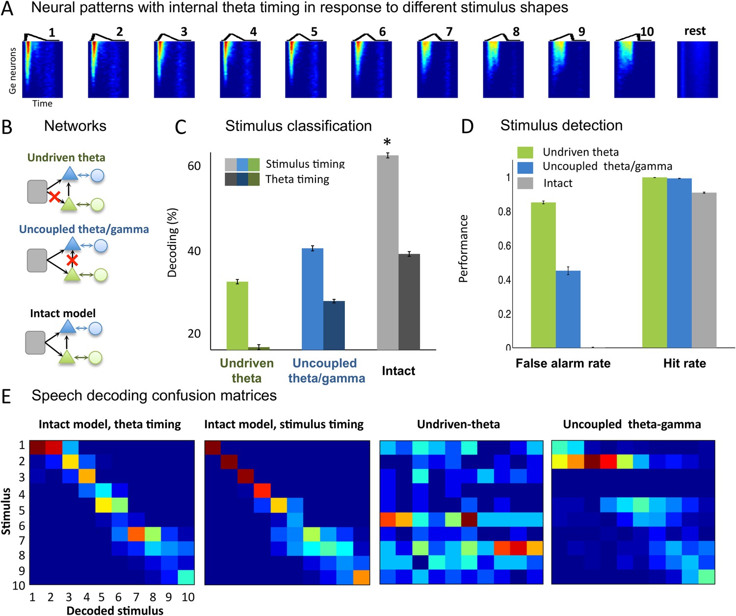
Sawtooth classification.
(A) Gamma spiking patterns in response to simple stimuli. The model was presented with 50 ms sawtooth stimuli, where peak timing was parameterized between 0 (peak at onset) and 1 (peak at offset). Spiking is shown for different Ge neurons (y axis) in windows phase-locked to theta bursts (−20 to +70 ms around the burst, x-axis). Neural patterns are plotted below the corresponding sawtooths. (B) Simulated networks. The analysis was performed on simulated data from three distinct networks: ‘Undriven-theta model’ (no speech input to Te units, top), ‘Uncoupled theta/gamma model’ (no projection from Te to Ge units, middle), full intact model (bottom). (C) Classification performance using stimulus vs. theta timing for the three simulated networks. The stimulus timing (light bars) is obtained by extracting Ge spikes in a fixed-size window locked to the onset of the external stimulus; the theta timing (dark bars) is obtained by extracting Ge spikes in a window defined by consecutive theta bursts (theta chunk, see Figure 3A). Classification was repeated 10 times for each network and neural code, and mean values and standard deviation were extracted. Average expected chance level is 10%. (D) Stimulus detection performance, for the intact and control models. Rest neural patterns were discriminated against any of the 10 neural patterns defined by the 10 distinct temporal shapes. (E) Confusion matrices for stimulus- and theta-timing and the two control models (using theta-timing code). The colour of each cell represents the number of trials where a stimulus parameter was associated with a decoded parameter (blue: low numbers; red: high numbers). Values on the diagonal represent correct decoding.
Figure 4 with 1 supplement
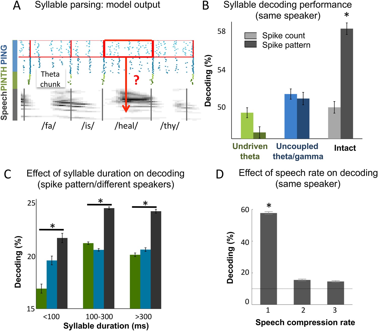
Continuous speech parsing and syllable classification.
(A) Decoding scheme. Output spike patterns were built by extracting Ge spikes occurring within time windows defined by consecutive theta bursts (red boxes) during speech processing simulations. Each output pattern was then labelled with the corresponding syllable (grey bars). (B) Syllable decoding average performance for uncompressed speech. Performance for the three simulated models (Figure 3B) using two possible neural codes: spike count and spike pattern. (C) Syllable decoding average performance across speakers, using the spike pattern code. Syllable decoding was optimal when syllable duration was within the 100–300 ms range, i.e., corresponded to the duration of one theta cycle. The intact model performed better than the two controls irrespective of syllable duration range. Chance level is 10%. Colour code same as B. (D) Syllable decoding performance for compressed speech for the intact model using the spike pattern code (same speaker, as in B). Compression ranges from 1 (uncompressed) to 3. Average chance level is 10% (horizontal line in the right plot).
Figure 4—figure supplement 1
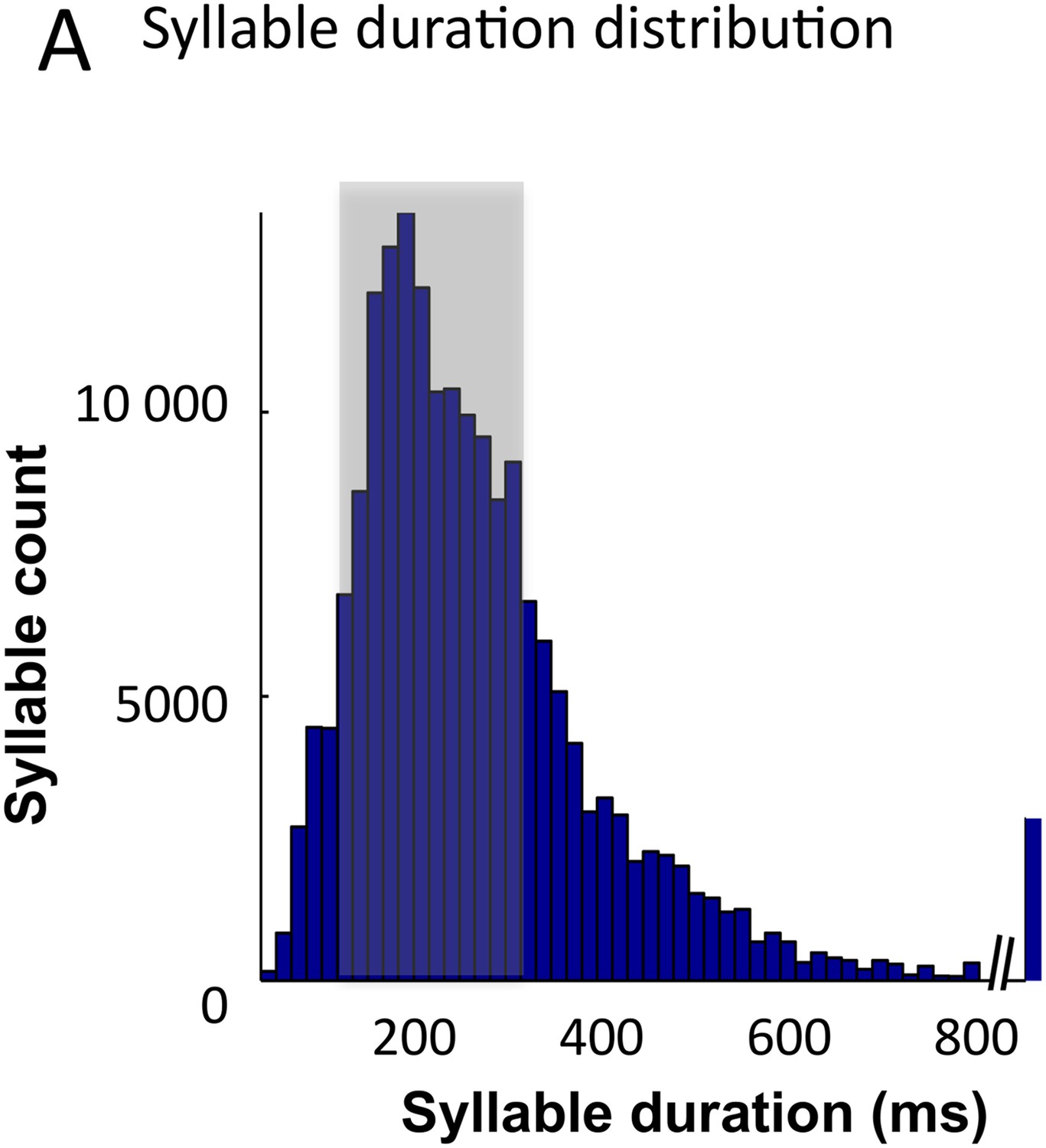
Syllable classification across speakers.
(A) Distribution of syllable duration across sentences and 462 speakers. The shaded area (100–300 ms) indicates region of maximal density. Extreme values probably correspond to ill-defined syllables.
Figure 5 with 1 supplement
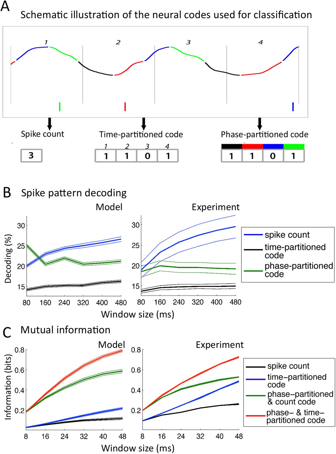
Comparison with encoding properties of auditory cortical neurons.
(A) Neural codes. Stimulus decoding was performed on patterns of Ge spikes chunked in fixed-size windows (the figure illustrates the pattern for one neuron extracted from one window). Spike count consisted of counting all spikes for each neuron within the window. Time-partitioned code was obtained in dividing the window in N equal size bins (vertical grey bars) and counting spikes within each bin. Phase-partitioned code was obtained by binning LFP phase into N bins (depicted by the four colours in the top graph) and assigning each spike with the corresponding phase bin. (B) Spike pattern decoding. (Left) Decoding performance across Ge neurons for the intact model using N = 8 bins for each code: spike count (black curve), time-partitioned (blue curve), and phase-partitioned codes (green curve). (Right) Data from the original experiment. Adapted from Kayser et al., 2012. (C) Mutual information (MI). (Left) Mean MI between stimulus and individual output neuron activity during sentence processing in the intact model for spike count (black curve), time-partitioned (blue line), combined count and phase-partitioned (green line) and combined time- and phase-partitioned codes (red line). (Right) Comparison with experimental data from auditory cortex neurons (adapted from Kayser et al., 2009).
Figure 5—figure supplement 1
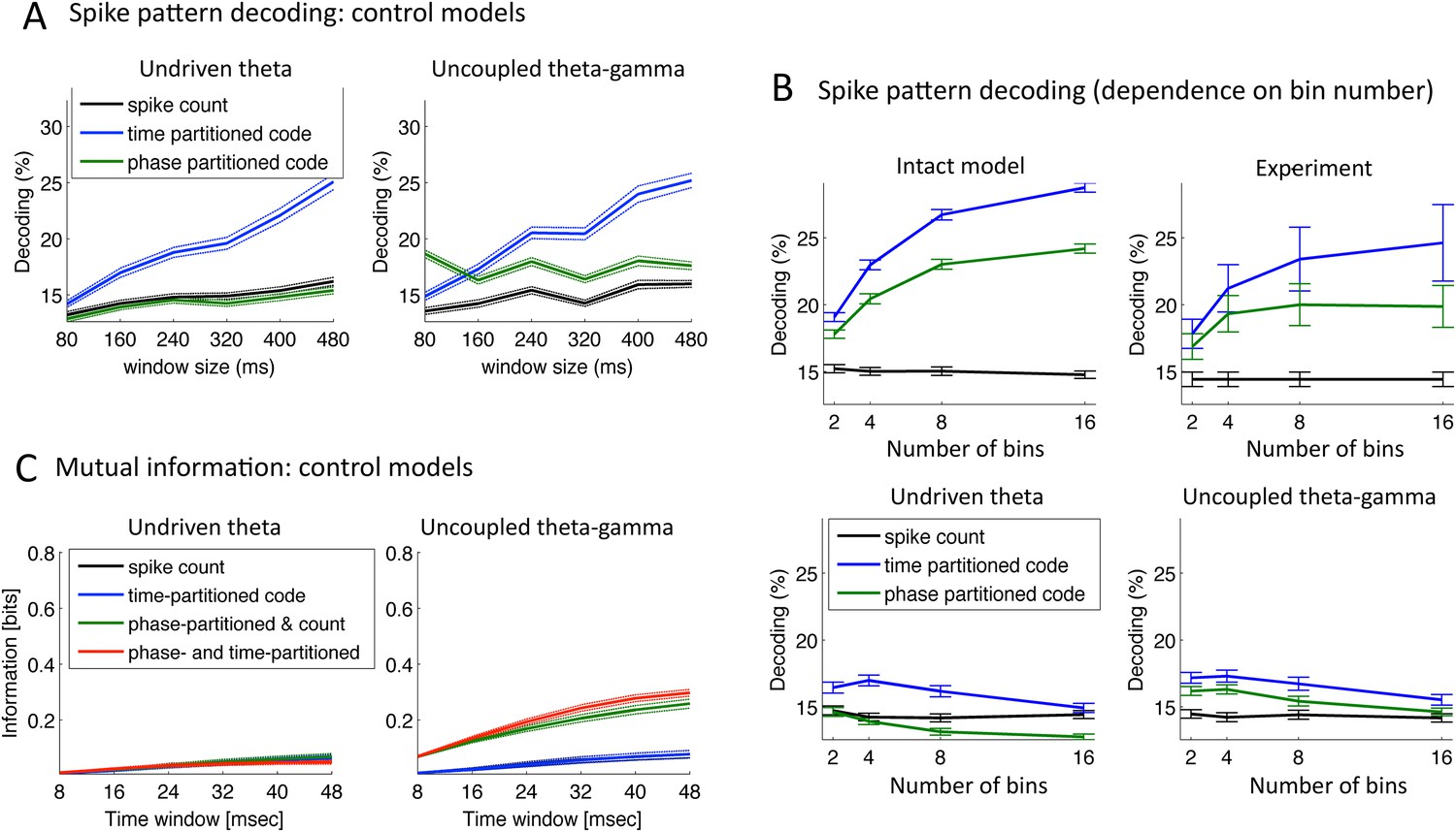
Speech decoding performance and MI (control models).
(A) Stimulus decoding performance for each neural code across Ge neurons for the control models (left:undriven theta; right: no theta–gamma connection): spike count (black line); time-partitioned neural code (blue line); phase-partitioned neural code (green line). (B) Stimulus decoding performance as a function of bin number, for all three variants of the model and experimental data. The number of bins used to partition the spikes was varied from 2 to 16, while the duration of the window was kept at 160 ms. Each dot corresponds to the average over 1000 different sets of stimuli and neuron (bars represent s.e.m.). Data from the original experiment, recording auditory cortex neurons from monkeys listening to naturalistic sounds. Experimental data are reproduced qualitatively by the intact model but not by the control model. Adapted from Figure 3E of Kayser et al., 2012. (C) Mutual Information (MI) between acoustic stimulus and individual Ge neurons for the control models (left: undriven theta; right: no theta–gamma connection): spike count (black line); time-partitioned neural code (blue line); phase-partitioned and spike count neural code (green line); phase- and time-partitioned neural code (red lines). Both control models display low MI values and fail to display the pattern of experimental data shown in Figure 5B.
Author response image 1
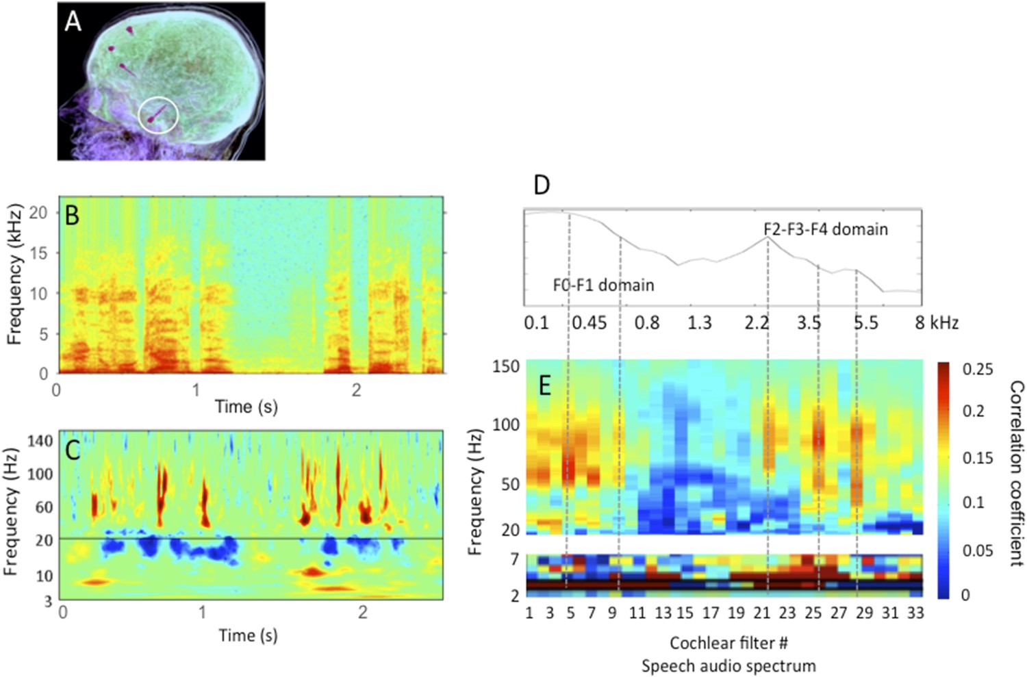
Human stereotactic EEG recording in auditory cortex.
A: the location of the electrode shaft, B: acoustic stimulus (one sentence); C: time-frequency representation of the cortical response in primary auditory cortex; D: spectrum of the stimulus in relation with E: the cross-correlation between stimulus (Hilbert transform of B) and cortical response for 33 different frequency bands (corresponding to 33 cochlear filters) spanning the speech audio spectrum up to 8 kHz. Note that the cross-correlation is broad-band in the theta range, but frequency specific in the gamma range, with peaks of correlation corresponding roughly to the energy peaks (speech formants). The data partly published in Morillon et al., 2012 and Giraud and Poeppel, 2012, and partly original.
Tables
Table 1
Full network parameter set
| Parameter | C | VTHR | VRESET | VK | VL | gL | |||
|---|---|---|---|---|---|---|---|---|---|
| Value | 1 F/cm2 | −40 mV | −87 mV | −100 mV | −67 mV | 0.1 | 5/NGe | 5/NGi | 0.3/NTe |
| Parameter | ||||||||
|---|---|---|---|---|---|---|---|---|
| Value | 0.2 ms | 4 ms | 0.5 ms | 5 ms | 2 ms | 20 ms | 3 | 1 |
Table 2
Optimal parameters for the LN model
| Parameter | DC | ||
|---|---|---|---|
| Value | 0.0748 | 1.433 | 0.4672 |
Table 3
Optimal parameters for the theta model
| Pars | ||||||||||
|---|---|---|---|---|---|---|---|---|---|---|
| Value | 0.282 A | 2.028 A | 24.3 | 30.36 | 15 | 1.25 | 0.0851 | 0.432 | 0.207 | 0.264 |
Download links
A two-part list of links to download the article, or parts of the article, in various formats.
Downloads (link to download the article as PDF)
Open citations (links to open the citations from this article in various online reference manager services)
Cite this article (links to download the citations from this article in formats compatible with various reference manager tools)
Speech encoding by coupled cortical theta and gamma oscillations
eLife 4:e06213.
https://doi.org/10.7554/eLife.06213


