Competing basal ganglia pathways determine the difference between stopping and deciding not to go
- University of Pittsburgh, United States
- University of Pittsburgh and Carnegie Mellon University, United States
- Carnegie Mellon University, United States
Figures
Figure 1
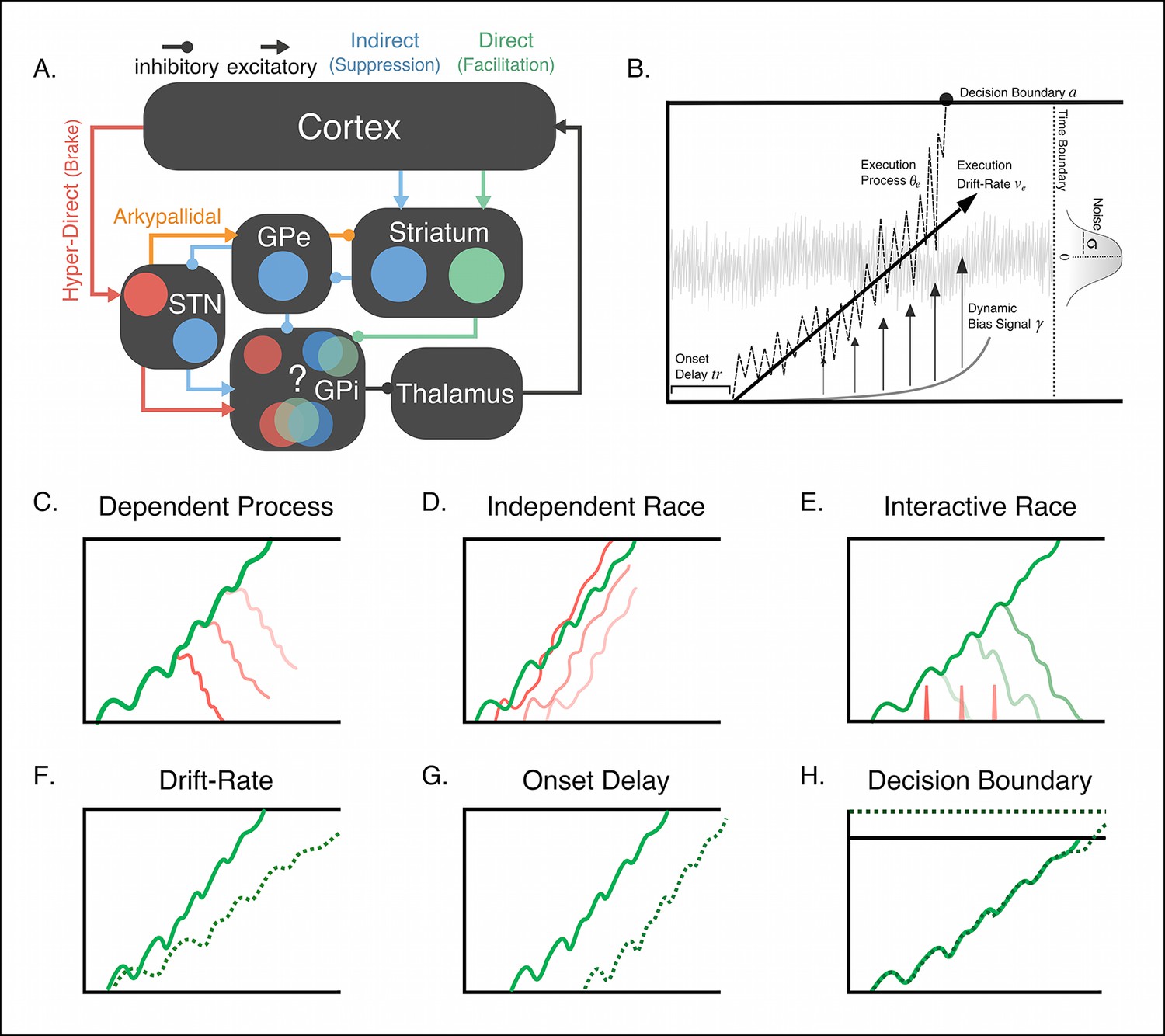
Conceptual framework of stopping and deciding not to go as separate but dependent processes.
(A) The organization of corticobasal ganglia pathways. Execution signals are relayed via the direct pathway (green connections) that result in a disinhibition of thalamic signals to cortex form the internal segment of the globus pallidus (GPi). Thalamic output can be suppressed by one of two major pathways. The indirect pathway (blue connections) increases inhibition of the thalamus via cortical signals terminating on striatal nuclei and relegated through the external segment of the globus pallidus (GPe). The hyperdirect pathway (red connections) quickly increase thalamic suppression via direct projections from the cortex to the subthalamic nucleus (STN). The question mark highlights the uncertainty as to whether the hyperdirect signals terminate on the same GPi neurons as the direct and indirect pathways. (B) Parameter structure of the general drift-diffusion process used in all model simulations and fits. For the reactive task (see Figure 1), we compared three models, a dependent process model (C), a traditional independent race model (D), and interactive race model (E). See main text for details on these models. For both reactive and proactive tasks, we compared three possible influences of context on the execution process: drift rate modulation (F), boundary shift modulation (G), and onset delay modulation (H). See main text for descriptions of each model.
Figure 2
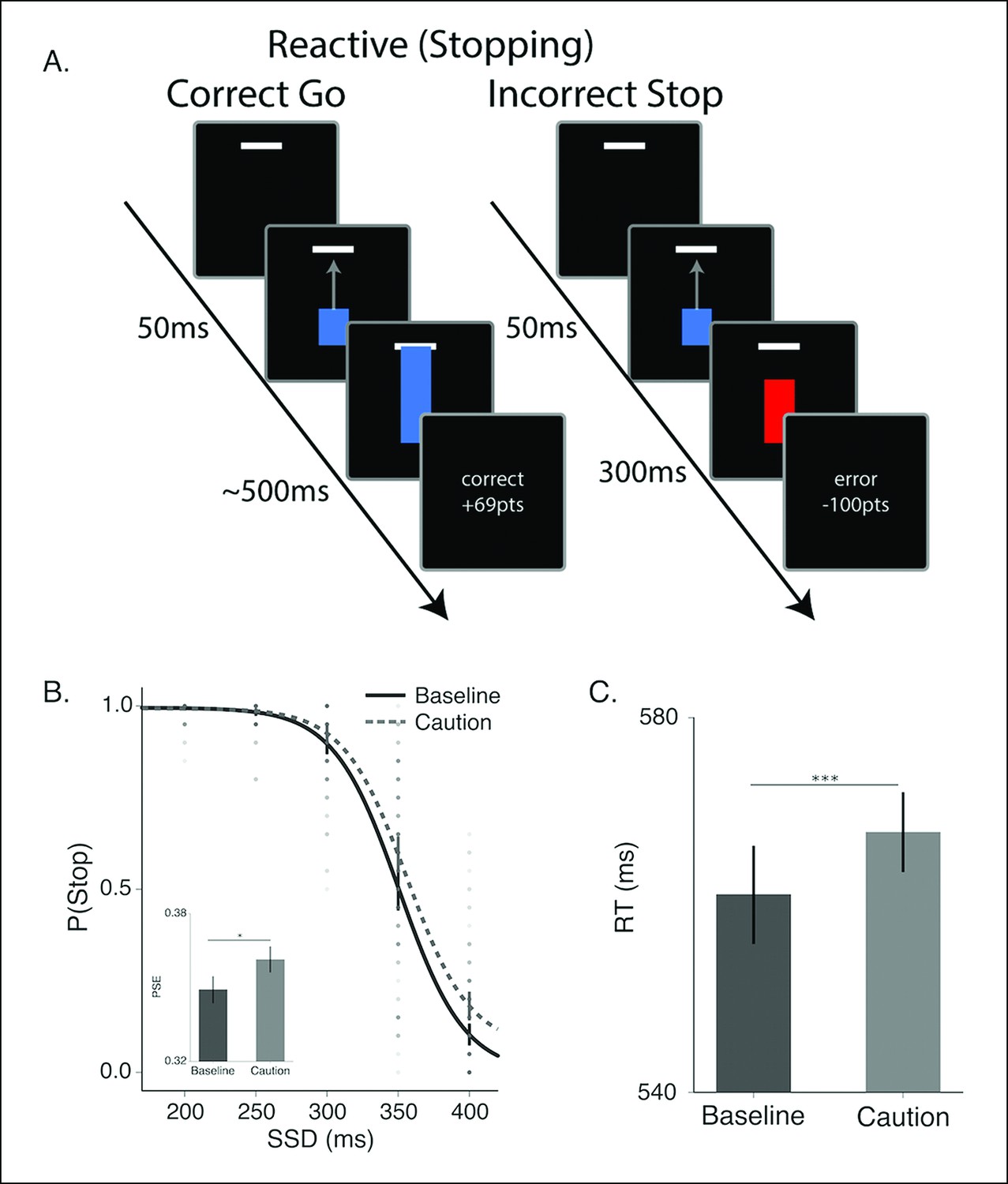
Reactive stopping task and behavioral results.
(A) Timeline of a go (left) and stop trial (right) in the reactive experiment. (B) Mean observed probability of stopping in the baseline (dark, solid) and caution (light, dotted) conditions; dots reflect individual subject means. As the stop-signal delay (SSD) increased, the probability of correctly stopping decreased. Inset in B shows the mean point of subjective equality (PSE) for both conditions. (C) Mean response times (RT) for the baseline and caution conditions. All error bars reflect the 95% confidence interval, * indicates p <0.05, *** indicates p <0.001.
Figure 3
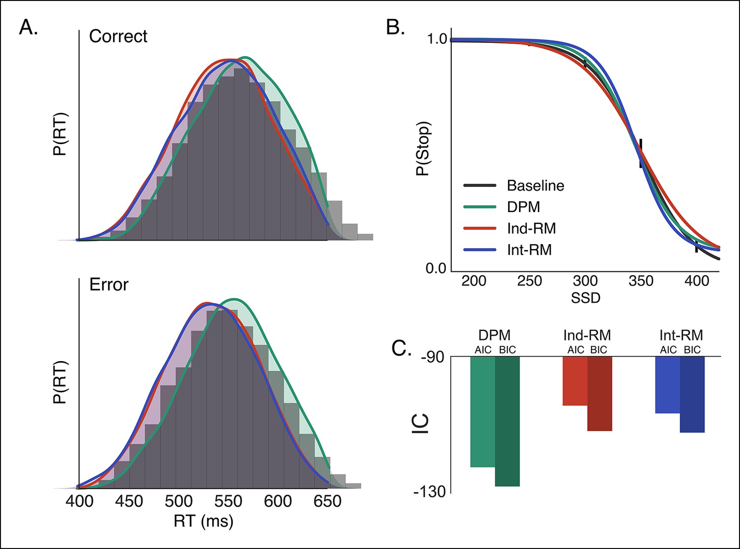
Comparison of reactive stopping models.
Fits of the three reactive models (Figure 1C–E) to behavioral data in the baseline condition, shown against (A) the histogram of RTs for correct (top) and incorrect (i.e., responses made on stop trials; bottom) trials and (B) the stop probability curve. Overall the dependent process model (DPM; green) explains speed and accuracy in the behavioral data (gray histograms in A, black line in B) better than the independent race model (Ind-RM; red) and interactive race model (Int-RM; blue). (C) Bars show the calculated AIC for each model. Error bars on behavioral data in B show the 95% confidence interval of the mean.
Figure 4 with 1 supplement
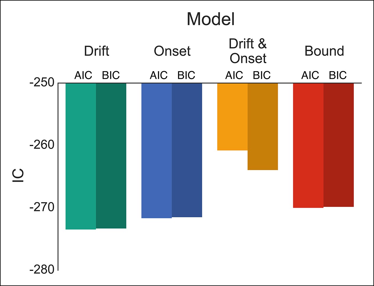
Comparison of modulation models in reactive task.
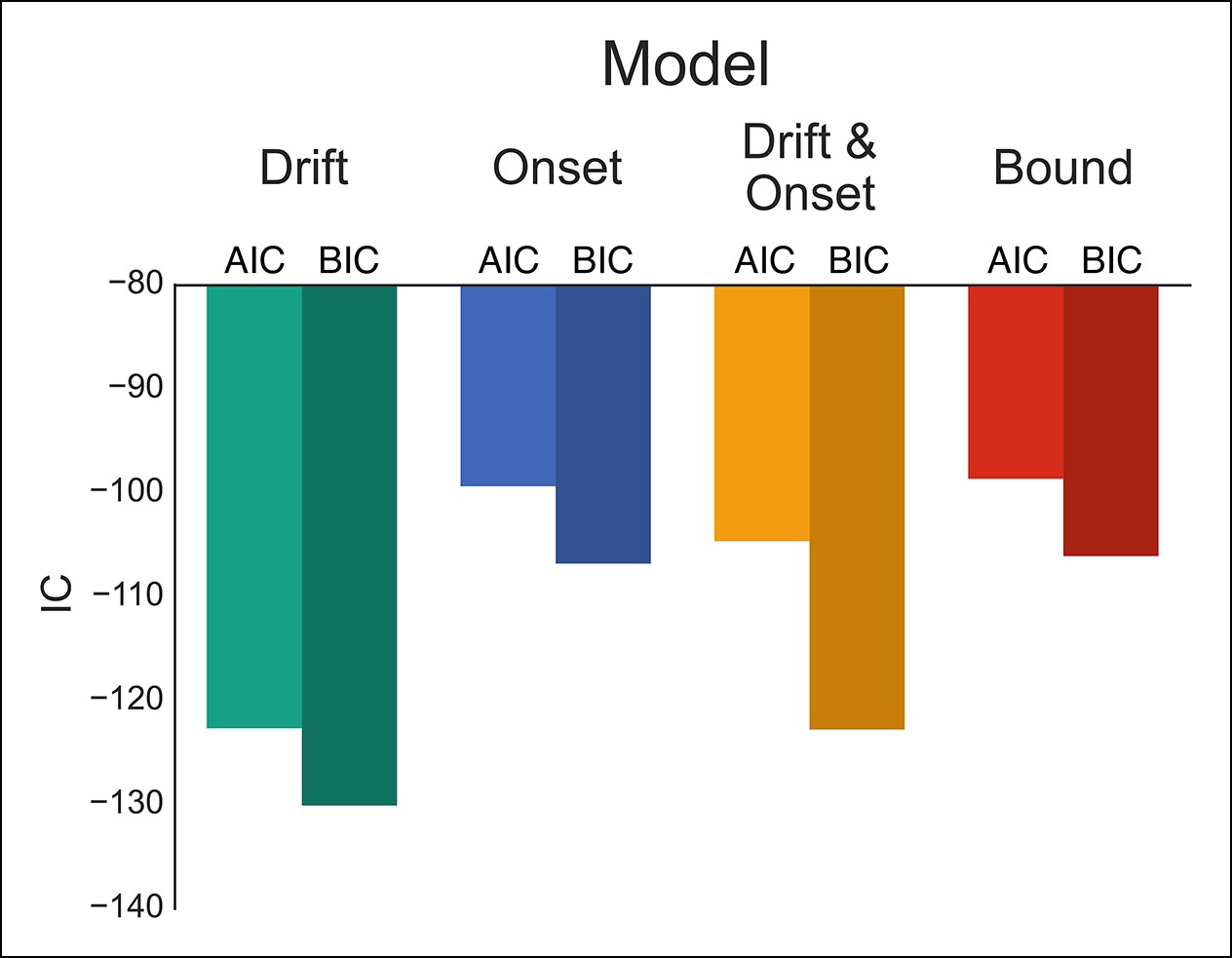
Goodness-of-fit measures for execution modulation models in reactive task. Bars show the estimated Akaike information criterion (AIC) and Bayesian information criterion (BIC) for the drift, onset, combined drift and onset, and boundary modulation models. The model with the lowest score, in this case the drift modulation model, is preferred.
Figure 4—figure supplement 1
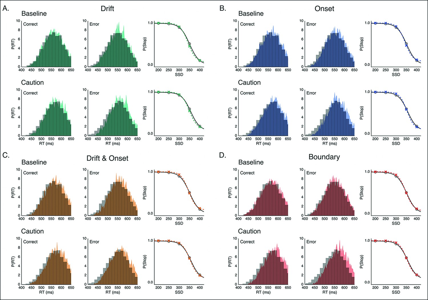
Model predictions of behavior in reactive task.
Example fits for modulation models on the execution process inthe baseline and caution conditions of the reactive task. Predicted RT distributions and stop accuracy are shown for the (A) drift-rate modulation model (green), (B) onset-modulation model (blue), (C) combined drift and onset modulation model (yellow), and (D) boundary modulation model (red). In each panel, RT distributions in the baseline (top) and caution (bottom) conditions are shown for correct (left) and error (right) trials. Empirical (gray, histograms) and model-predicted (color, probability density) RT distributions both reflect 1000 samples from a Gaussian kernel density estimate (bandwidth of. 01) based on the empirical and model simulated RT quantiles. The stop accuracy curve is plotted with model predictions (colored x’s) overlaid on empirical values (gray line, circles) for each of the five SSD conditions.
Figure 5 with 1 supplement
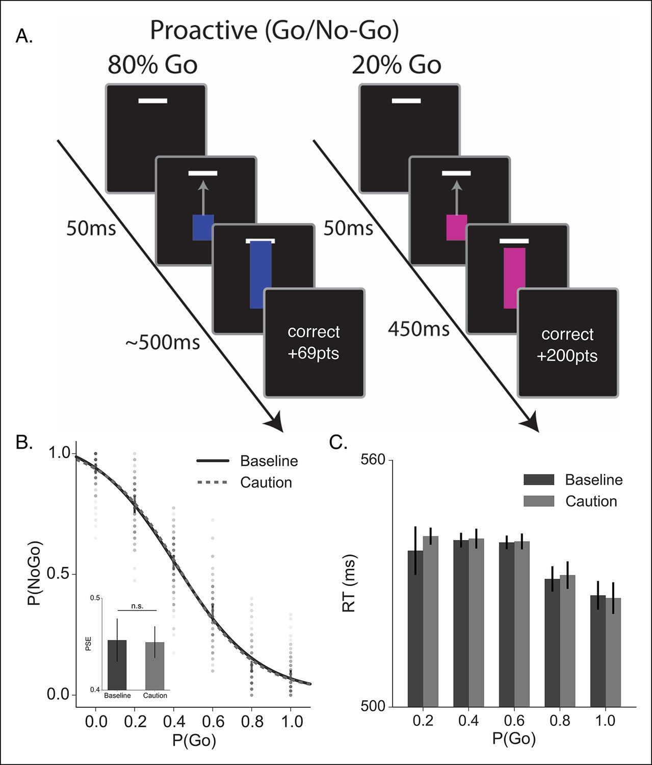
Proactive no-go decision task and behavioral results.
(A) Timeline of correct high (left) and low (right) go probability trials in the proactive task. The low probability example shows a trial in which a stop signal was presented. (B) Mean probability of making a no-go decision; dots reflect individual subject means and (C) mean reaction time plotted as a function of go trial probability in the baseline (dark, solid) and caution (light, dotted) conditions. Inset in B shows the mean point of subjective equality (PSE) for both conditions. All error bars reflect the 95% confidence interval; n.s. indicates a nonsignificant comparison at α of 0.05.
Figure 5—figure supplement 1
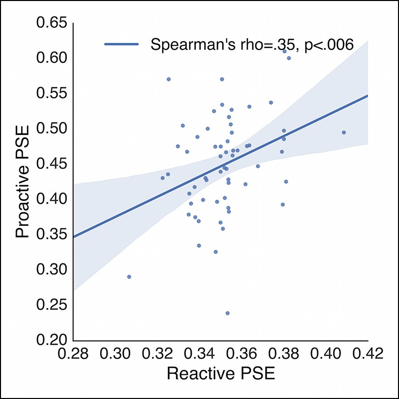
Subject-wise correlation of reactive and proactive control.
Correlation between the average PSEs in the reactive stopping curves and proactive no-go curves collapsed across baseline and caution conditions. Each point represents a single subject. PSE: point of subjective equality.
Figure 6 with 1 supplement
Comparison of modulation models in proactive task.
Goodness-of-fit measures for execution process modulation models in proactive task. Same plotting conventions as in Figure 4. As with the reactive experiment, the drift modulation model provided better fits to the proactive task data than the other models.
Figure 6—figure supplement 1
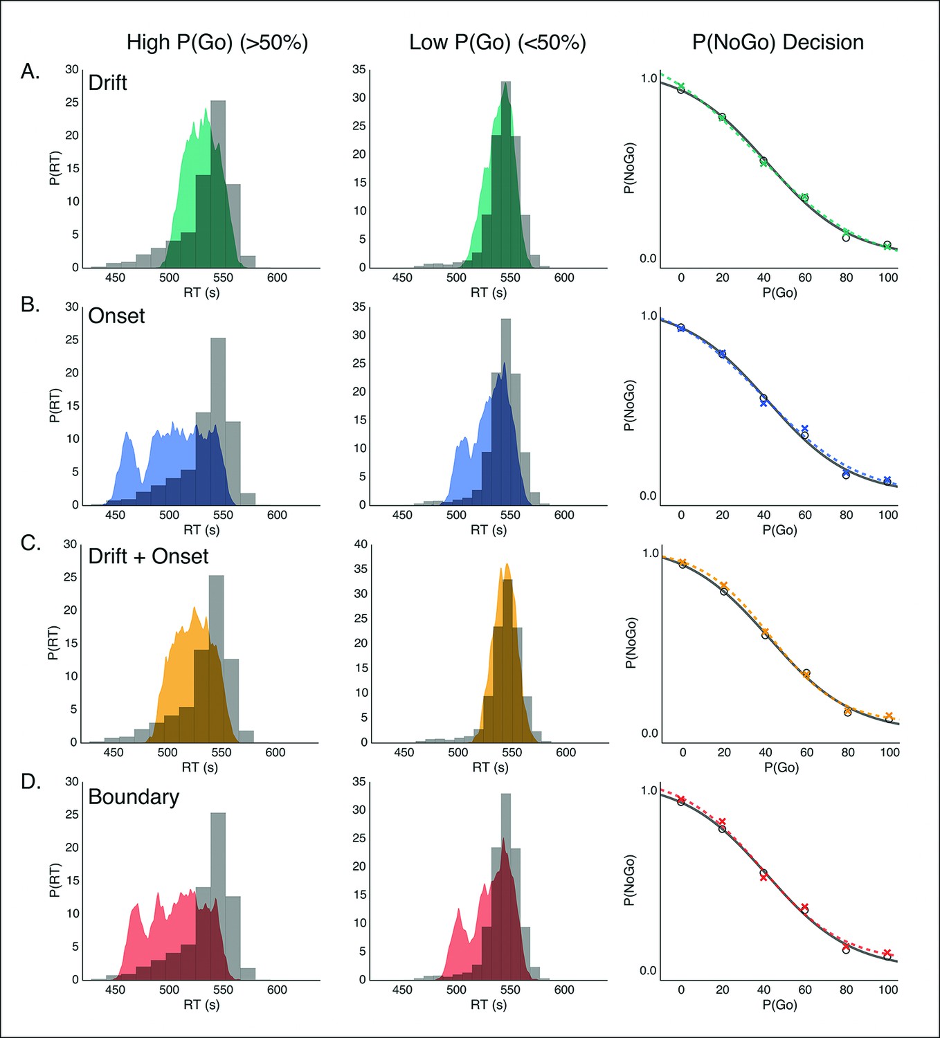
Model predictions of behavior in proactive task.
Predicted RT distributions and no-go probability curves in the proactive task for the drift modulation (green, A), onset modulation (blue, B), onset and drift modulation (yellow, C), and boundary modulation models (red, D). Empirical (gray) and kernel density estimates (same conventions as in Figure 4) for the RT distributions are shown for the high and low go trial probability conditions in the left and middle columns, respectively. Right column shows no-go probability curves for each go trial probability condition.
Figure 7
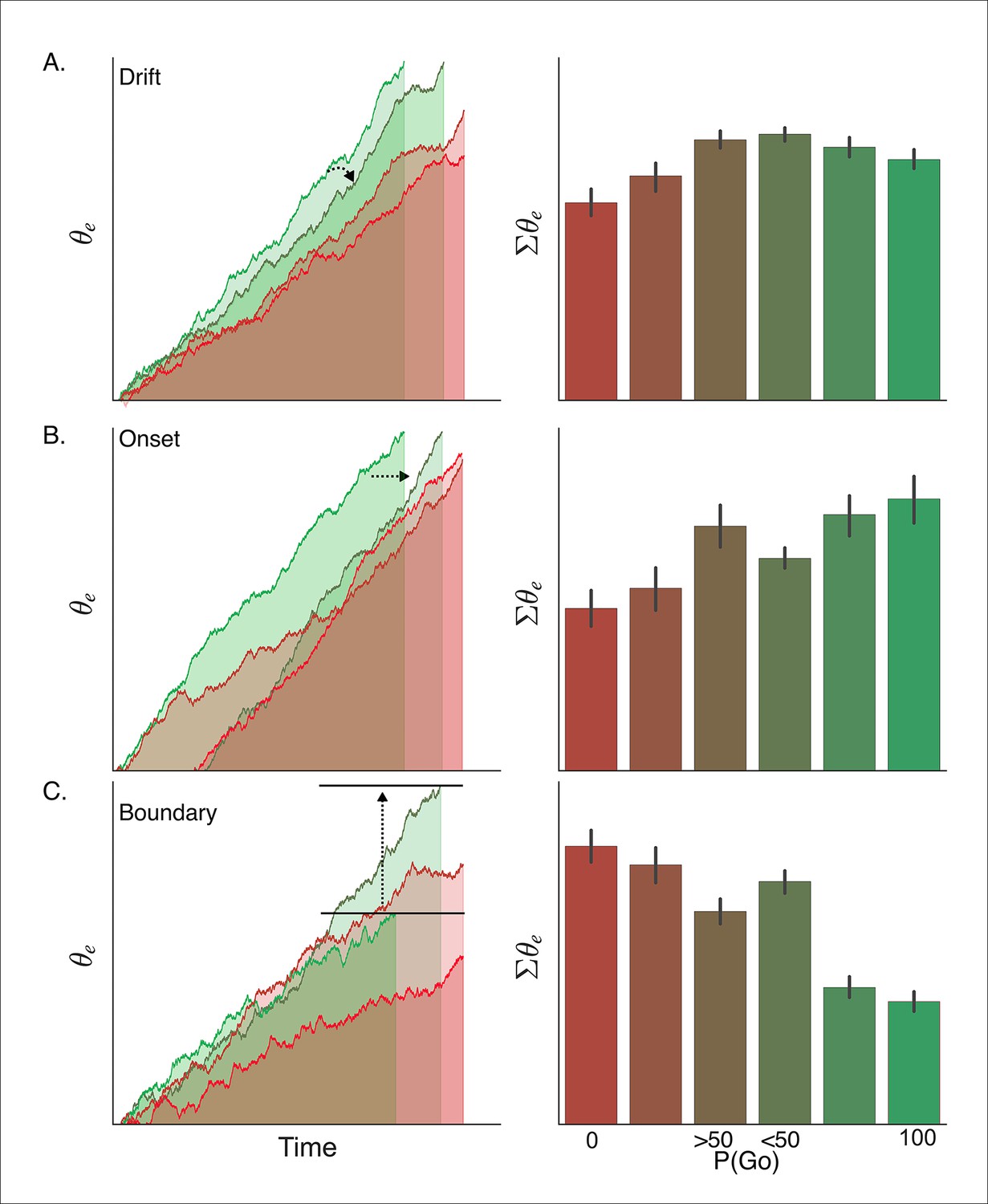
Simulated interaction between trial outcome and response expectation on BOLD activation.
Time-course of BOLD and mean activity in the proactive task predicted by the (A) drift modulation, (B) onset modulation, and (C) boundary modulation models. Time courses (left column) reflect the rise of the execution process (θe) on ‘go’ trials (left panels; green lines) and ‘no-go’ trials (right panels; red lines). Lighter colors reflect lower go probability conditions (go, <50%; no-go, 0%) and darker colors represent higher go probability conditions (go, 100%; no-go, >50%). The arrows in A and B show the pressure on the execution process with decreasing go trial certainty. The arrow and bars in C illustrate the shift in boundary height between high (bottom bar) and low (top bar) go trial probability conditions. Mean simulated BOLD responses (right column) are calculated as the cumulative sum of execution process across the full time course. This summation is reflected in the filled area under the curve in the traces in the left column. BOLD: blood oxygenation level dependent.
Figure 8 with 1 supplement
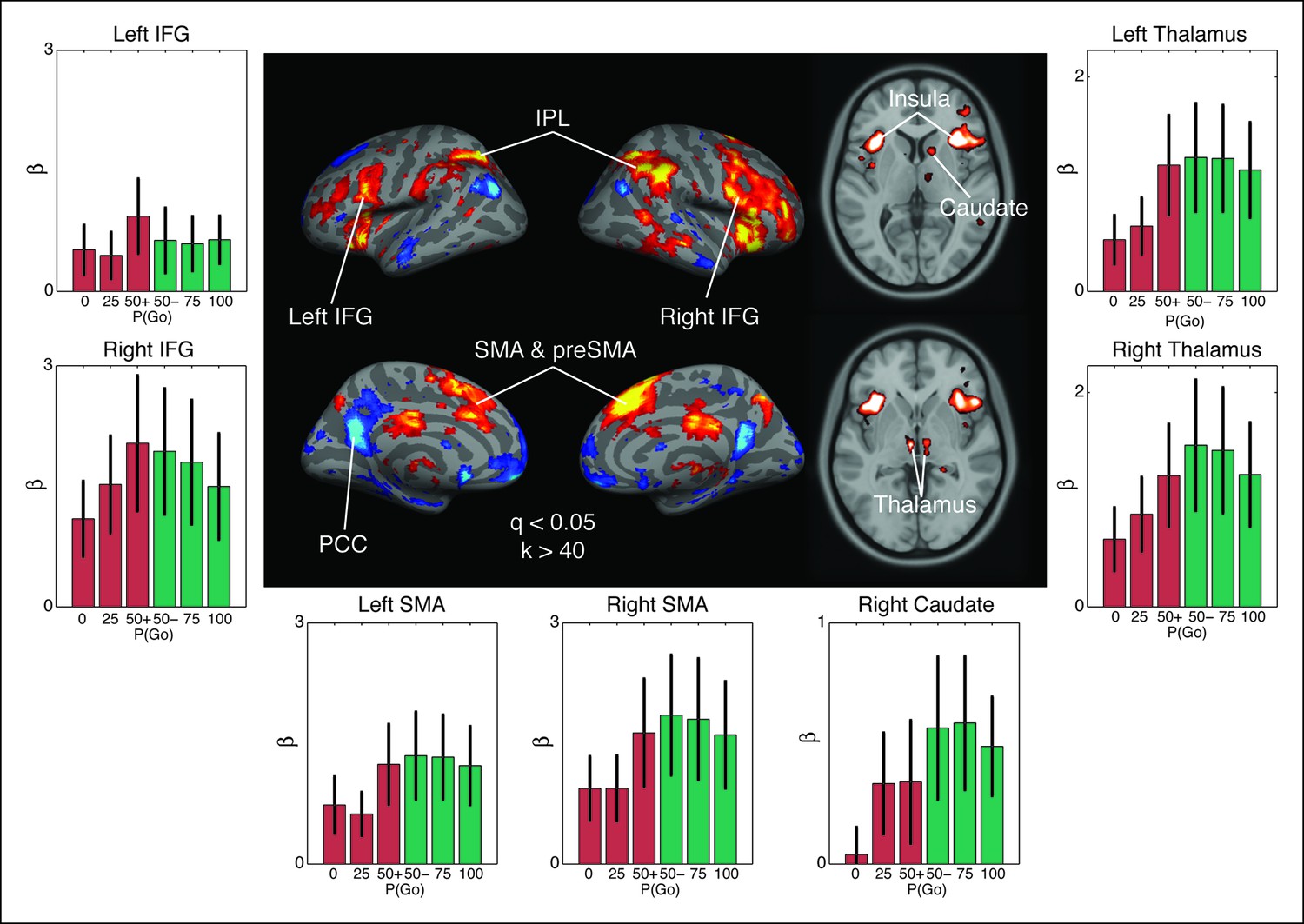
Observed interaction between trial outcome and response expectation on BOLD activation.
Contrast maps for the comparison of no-go responses, modulated by go trial probability, against modulated go responses in the proactive task (center panel). Warm colors show areas where the modulation was more positive during no-go trials than go trials. This is the direction predicted by the drift modulation model (Figure 7A). All voxels are corrected to a false discovery rate of 0.05 (i.e., q <0.05). Region of interest (ROI) clusters were thresholded to a minimum of 40 continuously connected voxels (i.e., k >40). The side and bottom panels show individual responses for the go trial probability condition in seven ROIs. Red bars illustrate BOLD responses during trials where no key press was registered (no-go trials) and green bars show BOLD fits to trials where a response was registered (go). BOLD: blood oxygenation level dependent; AMA: supplementary motor area; preSMA: pre-supplementary motor area; IFG: inferior frontal gyrus; IPL: inferior parietal lobule; PCC: posterior cingulate cortex.
Figure 8—figure supplement 1
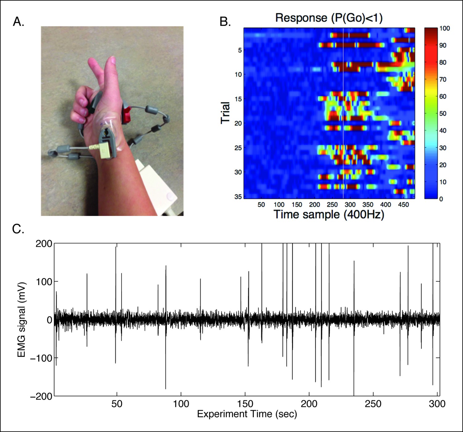
In-scanner EMG protocol.
(A) Example of modified EMG set-up using the in-house Siemens physiological monitoring unit for monitoring cardiac signals. The recording sensors were placed to estimate the electrical vector from the first dorsal interosseous (FDI) muscle of the responding right hand. (B) Trial-wise EMG responses detected for the trials where a response was made. Trials are time-locked to the start of the preparatory cue. White line indicates time in which the bar intersected the target. Recording for responses continued well after the end of the trial to identify late responses. (C) An example raw EMG signal from a single subject with peaks coinciding with finger movements.
Tables
Table 1
Reactive model parameter estimates and fit statistics. In the top panel, best fit parameter estimates for boundary height (a), onset delay (tr), execution drift rate (ve), braking drift rate (vb), dynamic bias gain (xb) are listed for each of the candidates reactive stopping models. Additionally, the stop signal onset delay (sso) was estimated for the interactive race model but was not included in the other models. The lower panel contains parameter estimates and fit statistics for the candidate models of contextual modulation between baseline and caution conditions of the reactive task. Parameters that were left free to vary between conditions contain two values, one estimate for the baseline condition and another estimate for the caution condition (see Model fitting for details regarding acquisition of constant parameters and optimization across conditions). In both panels, the last three columns show the χ2 as an absolute index of how well each model fit the data as well as the Akaike information criterion (AIC), and Bayesian information criterion (BIC) as complexity penalized goodness-of-fit measures. Lower values in all three measures imply a better fit to the data.
| Model | a | tr | ve | vb | sso | xb | χ2 | AIC | BIC |
| DPM | 0.534 | 0.174 | 1.266 | −0.990 | 0.878 | 0.0028 | −122.40 | −128.018 | |
| Ind-RM | 0.250 | 0.338 | 1.127 | 1.269 | 1.52 | 0.0075 | −106.652 | −112.270 | |
| Int-RM | 0.445 | 0.220 | 1.195 | 3.023 | 0.197 | 1.474 | 0.0069 | −104.379 | −111.815 |
| Drift | 0.536 | 0.178 | B: 1.289 C: 1.243 | −0.984 | 0.877 | 0.0051 | −273.459 | −273.301 | |
| Onset | 0.531 | B:0.171 C: 0.180 | 1.236 | −0.960 | 0.893 | 0.0054 | −271.651 | −271.492 | |
| Drift and onset | 0.538 | B: 0.173 C: 0.178 | B: 1.269 C: 1.247 | −0.989 | 0.858 | 0.0063 | −260.793 | −263.941 | |
| Bound | B: 0.525 C: 0.551 | 0.178 | 1.268 | -0.984 | 0.878 | 0.0057 | −269.994 | −269.835 |
-
DPM: dependent process model; Ind-RM: independent race model; Int-RM: interactive race model.
Table 2
Proactive model parameter estimates and fit statistics. Best fit parameter estimates for boundary height (a), onset delay (tr), execution drift rate (ve), and dynamic bias gain (xb) are listed for each of the proactive modulation models. For each model, free parameter (s) are named in the shaded column, followed by fitted estimates in each go trial probability condition in columns P0–P100, (see Model fitting for details regarding acquisition of constant parameters and optimization across conditions). The last three columns show the χ2 as an absolute index of how well each model fit the data as well as the Akaike Information Criterion (AIC), and Bayesian Information Criterion (BIC) as complexity penalized goodness-of-fit measures. Lower values in all three measures imply a better fit to the data.
| Model | a | tr | ve | xb | P0 | P20 | P40 | P60 | P80 | P100 | cXχ2 | AIC | BIC | |
| Drift | 0.487 | 0.292 | 1.563 | ve | 1.411 | 1.562 | 1.683 | 1.761 | 1.880 | 1.925 | 0.0022 | −122.65 | −130.08 | |
| Onset | 0.628 | 1.42 | 0.641 | tr | 0.182 | 0.161 | 0.134 | 0.117 | 0.084 | 0.076 | 0.0095 | −99.38 | −106.81 | |
| Drift and onset | 0.06 | 1.468 | ve | 0.831 | 0.970 | 0.968 | 0.979 | 0.932 | 1.079 | 0.0033 | −104.65 | −122.77 | ||
| tr | 0.515 | 0.506 | 0.492 | 0.479 | 0.451 | 0.463 | ||||||||
| Bound | 0.272 | 0.914 | 0.913 | a | 0.379 | 0.344 | 0.305 | 0.281 | 0.246 | 0.236 | 0.0099 | −98.65 | −106.09 |
Additional files
-
Supplementary file 1
Table of significant clusters for the no-go parametric minus go parametric contrast shown in Figure 8A.
Coordinates are centers of mass for the cluster in MNI-space. N is the number of voxels in each cluster. Values in the left six columns show average condition-wise (general linear model) GLM coefficients and standard deviation across subjects is in parentheses.
- https://doi.org/10.7554/eLife.08723.017
Download links
A two-part list of links to download the article, or parts of the article, in various formats.
Downloads (link to download the article as PDF)
Open citations (links to open the citations from this article in various online reference manager services)
Cite this article (links to download the citations from this article in formats compatible with various reference manager tools)
Competing basal ganglia pathways determine the difference between stopping and deciding not to go
eLife 4:e08723.
https://doi.org/10.7554/eLife.08723


