Testing sensory evidence against mnemonic templates
Figures
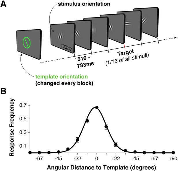
Task design and behavior.
(A) Each block began with the presentation of a target orientation, which observers maintained for the duration of a task block. Template presentation was followed by a serial stream of randomly oriented stimuli. Observers were asked to respond with a button press whenever the stimulus matched the template orientation. (B) Response frequency was highest for target trials, and dropped off sharply for non-targets with increasing angular distance between template and stimulus orientation. Error bars indicate standard error of the mean across observers. The black line denotes a von Mises distribution fit to the responses.
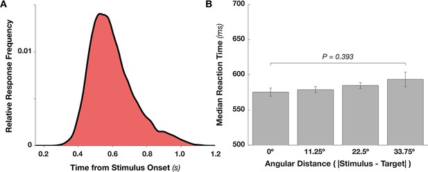
Reaction Time Distribution and Effects of Target Proximity.
(A) Distribution of reaction time frequencies (as a proportion of all responses), from stimulus onset (collapsing over hits and false alarms). Beginning around 400 ms after stimulus onset, response frequency rises rapidly up to approximately 550 ms, after which responses slowly taper off. (B) Target proximity (absolute angular distance between the stimulus and template angles) does not affect reaction time (F3,27 = 1.036, p = 0.393).
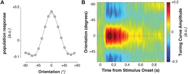
Stimulus-evoked population tuning curves.
(A) Average population tuning curve, 50–300 ms after stimulus onset. (B) Time-resolved population tuning curve, showing a sharp increase in the tuning curve slope shortly after stimulus onset, tapering off within 500 ms.
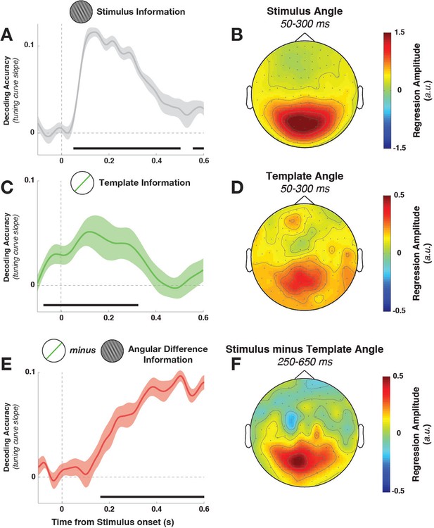
Task variable representation using population tuning curves (see Figure 2).
(A) Stimulus orientation was represented in the early visual response. We fit weights (using linear regression of stimulus orientation on the neural response) using all trials in all training blocks and estimated virtual channel responses in the test block. Orientation-specific coding was estimated by calculating the linear slope of the tuning curve (between 0° and 90°). Consistent positive slopes indicate orientation selectivity at a given time point. Shading indicates between-subject standard error of the mean. Black bars denote significant time points (cluster-corrected). (B) Univariate sensitivity for stimulus orientation, calculated at each sensor and time point. Topography shows the shuffle-corrected orientation sensitivity (z-scored against a distribution generated from permuting stimulus orientations 1000 times), averaged across sensor triplets (two orthogonal planar gradiometers and one magnetometer) and across the stimulus-decoding window. Color coding denotes the z-score, averaged across observers. (C) Tuning curve slope and topography (D) for template orientation sensitivity. E and F show the same analyses, sorting trials by the angular distance between template and stimulus (i.e., the decision value).
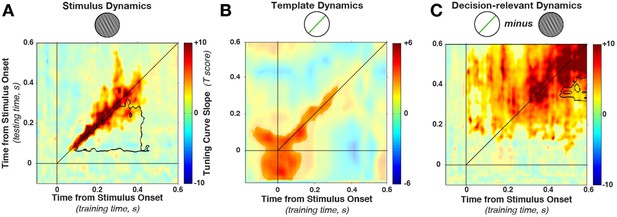
Cross-temporal generalization of orientation decoding.
(A) Tuning curve amplitude for stimulus orientation, estimated by calculating weights at one time point and applying them to test data at all time points in a trial. While decoding is consistently high along the diagonal (in the time window that contains significant stimulus information, between 52 and 544 ms, significant cluster indicated by color saturation/opacity), the slope drops sharply at off-diagonal train-test time coordinates. This indicates that the discriminative patterns are not consistent across time—rather they change rapidly, even while the stimulus can be readily decoded (i.e. off-diagonal decoding is significantly lower than on-diagonal decoding, black outline). B and C show the same analyses as in A, but sorting all trials by the template angle and the decision-relevant angular distance, respectively.
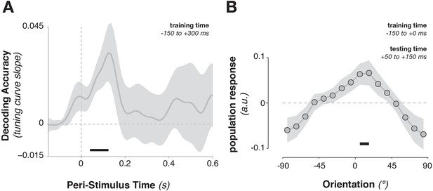
Cross-generalization from template-discriminative patterns to stimulus-discriminative patterns.
(A) Calculating tuning-curve weights relative to the template orientations in a training data set (in window from –150 to +300 ms around stimulus onset), applying these weights on test data, and sorting them relative to the stimulus orientation, showed decoding early after stimulus onset that quickly returned to baseline. (B) Calculating population weights only on the pre-stimulus period (with respect to the template orientations) yielded a population tuning curve with a significant peak around the presented stimulus orientation (e.g. a significant peak above the average response around 0º, and a significant positive tuning curve slope between ± 90º and 0º). Shading indicates the standard error of the mean. Black bars indicate significant time points or orientations (p < 0.05).
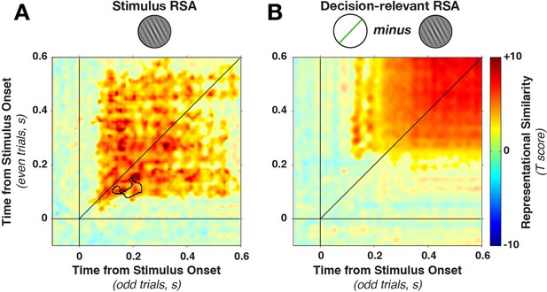
Cross-temporal generalization of representational similarity.
(A) Pearson correlations between stimulus-orientation-sorted distance matrices, calculated at different time points and on independent data sets. Color saturation shows significant cluster at the group level (permutation test). The cluster extends off the diagonal in a square, indicating substantial cross-temporal generalization. In addition, there is a small dynamic cluster (black outline), meaning that pairs of time points within the black outline showed significantly lower correlations than their corresponding time points on the diagonal (even though they were still significantly greater than 0). (B) shows the same analysis as in A, but sorting all trials by the decision-relevant angular distance. There were no significant dynamic clusters. RSA, representational similarity analysis.
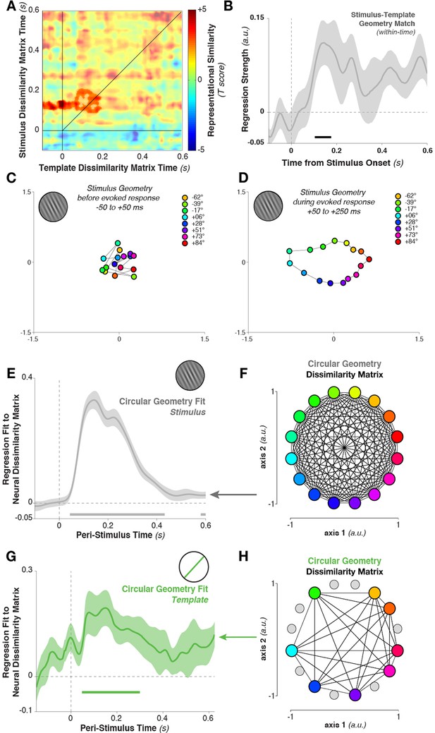
Geometry of stimulus and template coding.
(A) The representational similarity structures between template- and stimulus-ordered responses were significantly correlated in the early stimulus-processing window (saturated colors indicate significant cluster). (B) The within-time comparison also showed a significant correlation in the representational similarity structure from 104 to 176 ms. Values correspond to the mean regression coefficient across all observers. Shading is between-subjects standard error of the mean. (C) Multi-dimensional scaling of the distances between stimulus orientations was not visible before stimulus onset. (D) Shortly after stimulus onset, the circular structure indicated that responses used a circular geometry. (E To quantify the representational structure over time, we fit (using regression) to the neural distance matrix between all angles (16 different angles, split randomly into two sets of trials, resulting in a 32×32 distance matrix of Mahalanobis distances) the distance matrix of a 16-point circular simplex, shown in (F). (G) Similarly, relationships between the eight template orientations fit a circular structure, particularly around stimulus onset time. (H) An example of a simplex from one session, with the eight chosen template angles highlighted in color, and the eight stimulus orientations which were never targets shown in gray.
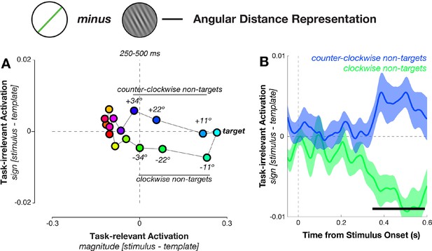
Geometry of response-related coding.
(A) Dissimilarity structure of angular distances. Data dimensionality was reduced using PCA, and weights calculated between sensor activity and different task variables using independent training data. Mean responses for each angular distance, calculated using the left-out data, were then projected via the calculated weights onto the task axes (the magnitude and sign of the angular distance). Since the task relevance of a particular angular distance was defined solely by its magnitude, projections onto the sign axis measured sensitivity to task-irrelevant signed differences between conditions. Prior to decision onset (250–500 ms after stimulus onset), the neural geometry is elliptical: in addition to conditions separating along the target-relevant magnitude axis (horizontal), near non-targets separate along the task-irrelevant sign axis (vertical). (B) Task-irrelevant coding emerges approximately 350 ms after stimulus onset. Time courses for the three nearest non-targets (11º, 22º, 34º offset from target angle) separate along the task-irrelevant axis, depending on whether they are clockwise or counterclockwise to the target.
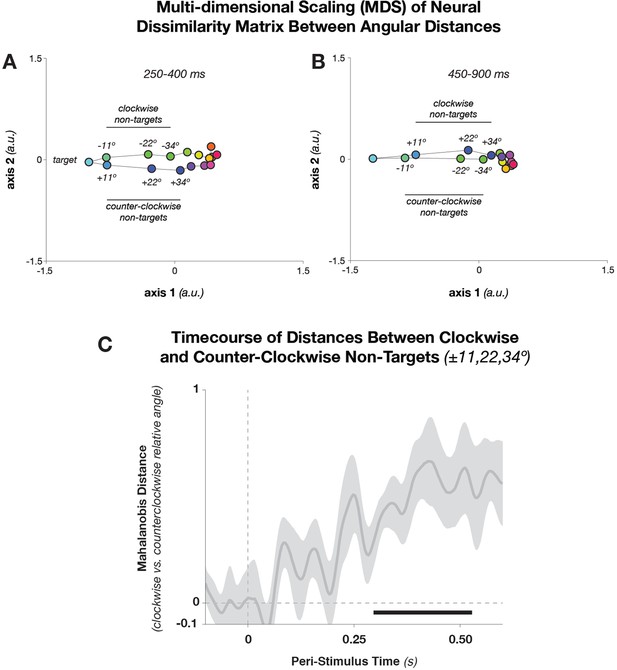
Multidimensional Scaling and Pairwise Mahalanobis distances between Angular Distances.
(A) Dissimilarity structure of angular distances. We used MDS, which maps the multidimensional (32× 32) Mahalanobis distance matrix between target-relative angles into two dimensions. During relatively early stimulus processing (250–400 ms after stimulus onset), geometry is elliptical—that is, in addition to conditions separating along the target-relative axis (horizontal), conditions separate along a task-irrelevant axis (vertical). During later processing stages (B: 450–900 ms), the task-related axis accounts for most of the condition differences. Since MDS is rotation-invariant, the solution in B happens to have flipped axis 2, without affecting the geometrical relationship between points. (C) Mahalanobis distances (shuffle-corrected) between trials with equal target proximity, but different direction (i.e., clockwise vs. counter-clockwise deviations of the stimulus angle, with respect to the template angle). The figure shows the mean z-score (with respect to 250 random permutations of the trial labels) of pairwise distances between equal target proximities, averaged over the pairs ± 11.25º, ± 22.5º, and ± 33.75º. Shading indicates standard error of the mean. The black bar denotes significant time points (p<0.05, cluster-corrected). MDS, multi-dimensional scaling
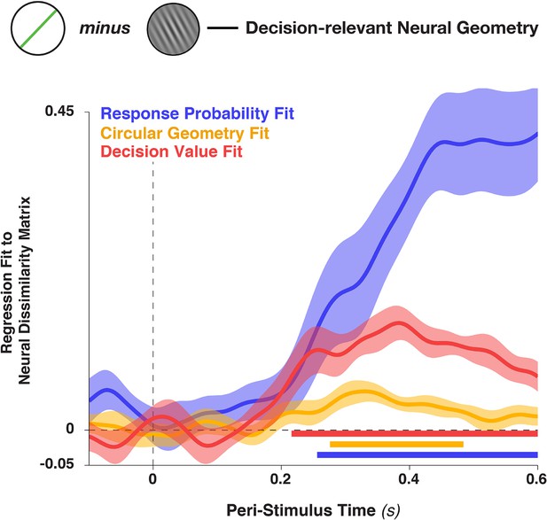
Figure is identical to Panel 8c, but includes in the graph the fit to the distance matrix provided by the linear decision value (i.e., the unsigned target proximity, stimulus—target ).
This variable was also included in the analysis described in the main text, but omitted from Figure 8C for clarity (since it a nuisance variable). Shading indicates standard error of the mean and colored bars at the bottom denote significant time points for each regressor (p<0.05, cluster-corrected).
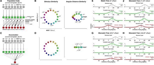
Neural Population Model.
(A) Probabilistic population code model architecture. (B) Dissimilarity structure of responses in the stimulus layer (left panel) and the decision layer (right panel). (C) Accumulator model architecture. In contrast to the population code, decision value here is represented only in a single node (red unit in the decision layer). Otherwise, the architectures are identical. (D) Dissimilarity structure of responses in the accumulator model. While responses in the stimulus layer are identical in both cases, the decision layer differs from the population code model, in that the magnitude, but not the direction, of angular differences between stimulus and template, is represented. (E) Model response on an exact template match trial. (F–H) Model responses on mismatch trials.


