Mapping residual transmission for malaria elimination
Figures
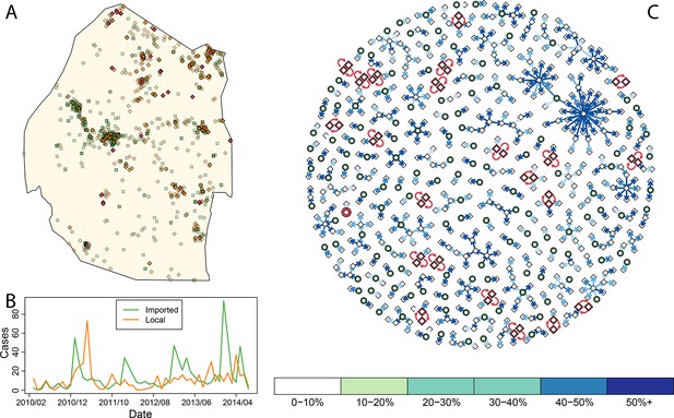
Consensus network plot of causal links.
Panel A: Swaziland imported and local malaria cases (green squares and orange diamonds, respectively) are plotted spatially. Local case pairs identified as putative orphaned chains are indicated by red diamonds. A solitary local case also identified as an orphan is identified as a red diamond within a circle. Panel B: Swaziland imported (green line) and local (orange line) malaria cases are plotted in time, aggregated by month. Panel C: The final consensus network plot is displayed. Local cases are plotted as diamonds and imported cases as green circles. The color of each link corresponds to the “strength” of the connection as measured by the number of parameter sets where that link was identified as optimal. Imported cases that were not found to be the “most likely” parent of a local case are not displayed.
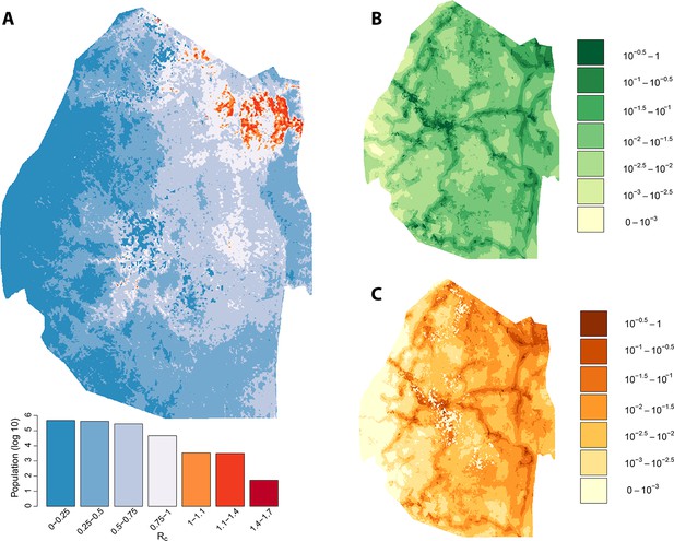
Vulnerability, receptivity and malariogenic potential.
Panel A: Extrapolated Rc values for Swaziland using a zero-inflated negative binomial regression. Areas in orange to red indicate locations where Rc is greater than unity. The legend doubles as a histogram indicating the number of individuals (on a log10 scale) that live within each range of Rc values. Panel B: Extrapolated importation probabilities for Swaziland using a logistic regression. Panel C: Malariogenic potential for Swaziland calculated as the product of Rc and the probability of importation.
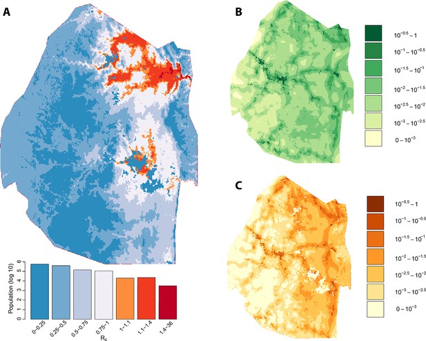
Vulnerability, receptivity and malariogenic potential (2010-6/2012).
Panel A: Extrapolated Rc values for Swaziland using a zero-inflated negative binomial regression. Areas in orange to red indicate locations where Rc is greater than unity. The legend doubles as a histogram indicating the number of individuals (on a log10 scale) that live within each range of Rc values. Panel B: Extrapolated importation probabilities for Swaziland using a logistic regression. Panel C: Malariogenic potential for Swaziland calculated as the product of Rc and the probability of importation.
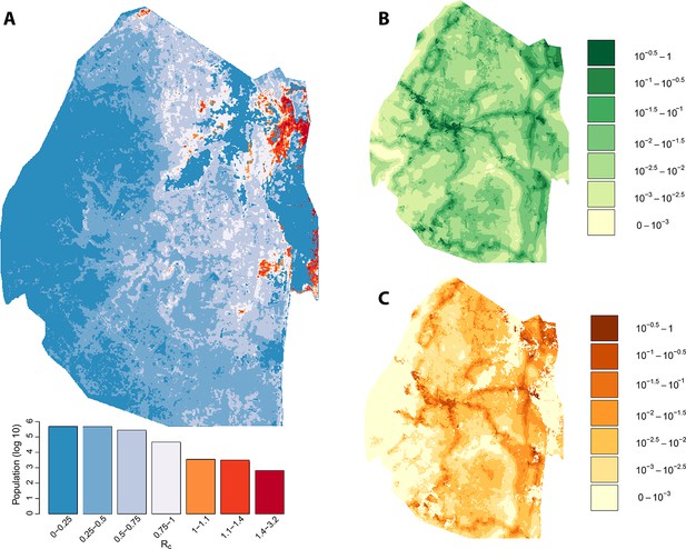
Vulnerability, receptivity and malariogenic potential (7/2012-2014).
Panel A: Extrapolated Rc values for Swaziland using a zero-inflated negative binomial regression. Areas in orange to red indicate locations where Rc is greater than unity. The legend doubles as a histogram indicating the number of individuals (on a log10 scale) that live within each range of Rc values. Panel B: Extrapolated importation probabilities for Swaziland using a logistic regression. Panel C: Malariogenic potential for Swaziland calculated as the product of Rc and the probability of importation.
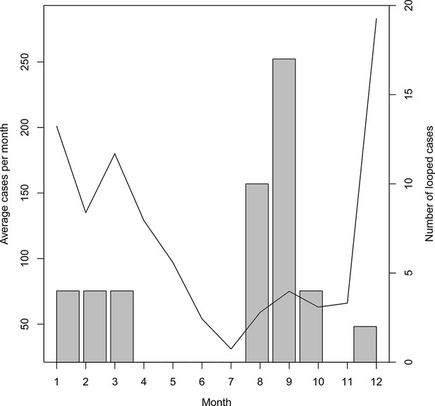
Timing of ‘orphan’ cases.
The average number of cases per month and total occurrence of looped (or ‘orphaned’ cases) are plotted against month.
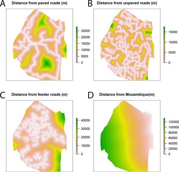
Spatial covariates for malaria receptivity regression.
The four significant covariates for the malaria receptivity regression were (A) distance from paved roads, (B) distance from unpaved roads, (C) distance from feeder roads, and (D) distance from Mozambique. All distances were in meters.
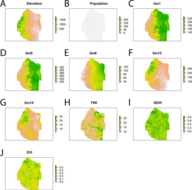
Spatial covariates for malaria importation regression.
The ten significant covariates for the malaria importation regression were (A) elevation, (B) population, (C) annual mean temperature (bio1 - http://www.worldclim.org/bioclim), (D) maximum temperature of the warmest month (bio5 - http://www.worldclim.org/bioclim), (E) minimum temperature of coldest month (bio6 - http://www.worldclim.org/bioclim), (F) precipitation of the wettest month (bio13 - http://www.worldclim.org/bioclim), (G) precipitation of driest month (bio14 - http://www.worldclim.org/bioclim), (H) TWI, (I) normalized difference vegetation index, and (J) enhanced vegetation index.
Tables
Zero-inflated negative binomial regression summary.
| Factor (source) | Count model coefficient | Zero-inflated coefficient |
|---|---|---|
| Intercept | 7.686407 | 1642.7199 |
| Elevation (m) (http://www.worldclim.org/bioclim) | −0.0026 | −0.65197 |
| Population (http://www.worldpop.org.uk/) | −0.017571 | −0.01190 |
| Annual Mean Temperature (0.1°C) (http://www.worldclim.org/bioclim) | 0.141979 | 30.70232 |
| Max Temperature of Warmest Month (0.1°C) (http://www.worldclim.org/bioclim) | −0.113297 | −23.66837 |
| Min Temperature of Coldest Month (0.1°C) | −0.029091 | −10.04161 |
| Precipitation of Wettest Month (mm) (http://www.worldclim.org/bioclim) | 0.008032 | 0.50592 |
| Precipitation of Driest Month (mm) (http://www.worldclim.org/bioclim) | −0.108767 | 12.04175 |
| TWI | −0.024820 | −4.02392 |
| NDVI (https://landsat.usgs.gov/) | 2.461314 | −159.39390 |
| EVI (https://landsat.usgs.gov/) | −3.732795 | 82.72595 |
| Log(theta) | −0.613861 | NA |
GAM logistic regression summary.
| Factor | edf | Chi.sq | p-value |
|---|---|---|---|
| Population (http://www.worldpop.org.uk/) | 6.729 | 688.01 | <2e-16 |
| Paved roads (source: country) | 5.909 | 172.49 | <2e-16 |
| Unpaved roads | 1.002 | 15.88 | 6.88e-5 |
| Feeders roads | 6.499 | 50.37 | 3e-8 |
| Distance to Mozambique (http://www.fao.org/geonetwork/srv/en/main.home) | 7.516 | 75.27 | 1.04e-12 |


