Active machine learning-driven experimentation to determine compound effects on protein patterns
Figures
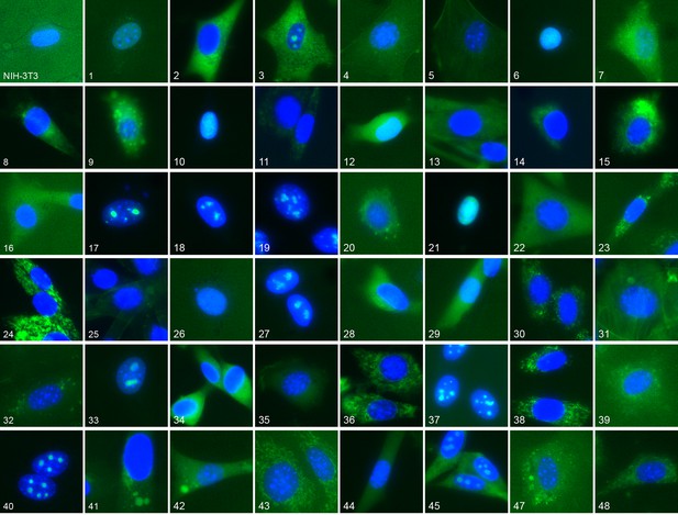
Representative location patterns of the CD-tagged clones.
Images of EGFP (green) and Hoechst 33,342 (blue) fluorescence were acquired at 40x with an automated widefield microscope (see Materials and methods). Each panel is independently contrast stretched. The identities of the tagged gene for each clone are listed in Supplementary file 1. Clone order is random with respect to location pattern. The untagged NIH 3T3 (upper left) was assigned as clone 46.
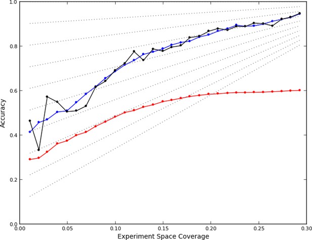
Accuracy of active learning.
The performance of the active learner (black line) generally increased superlinearly as more data were acquired. Hypothetical models (dotted gray lines) with fixed generalization accuracy have constant slopes and are displayed for reference (10% to 90% rates as isoclines). The initial model poorly generalized (~45%) while the final model learned at round 30 (29% experiment space coverage) had ~75% generalization accuracy and 92% overall accuracy. A regression model based on unique experiment coverage (blue line, see main text for details) qualitatively explains the observed learner performance. Using this coverage model, an estimate of expected accuracy for random learning was constructed (red line, see main text for details); the final accuracy difference between the active learner and random learning is ~40%.
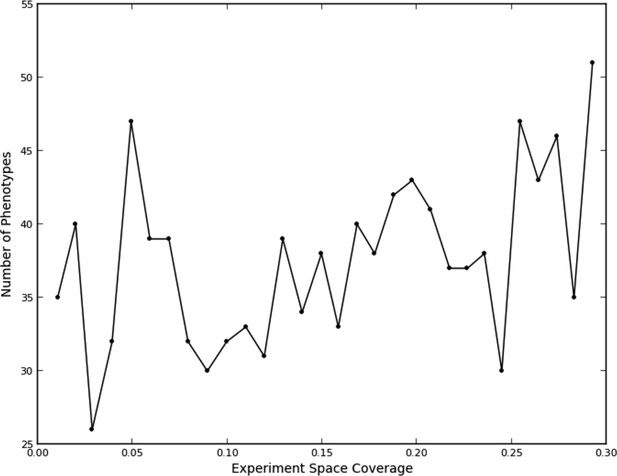
Number of phenotypes identified at each round in the learning process.
https://doi.org/10.7554/eLife.10047.007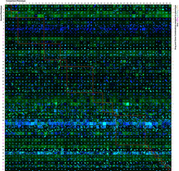
Contrasts between phenotypes identified by the active learner.
The last actively learned model identified 51 'phenotypes,' each phenotype of which is defined by a set of imaged fields. To independently assess the extent to which these phenotypes were different, a logistic regression classifier was trained to distinguish the actively learned phenotypes and evaluated by cross-validation; the classifier was able to distinguish all 51 phenotypes in fields not used for training with 75% accuracy. To give a sense of the spread of each phenotype, a randomly chosen cell from a field in the source phenotype (row) that had the median classification accuracy against another phenotype (column) is shown; this field that is chosen can be considered representative of the source phenotype when considered relative to the other phenotype. In this way, visually across a row one sees examples from each phenotype reflective of differences between it and other phenotypes. Phenotypes have been reindexed (Supplementary file 2 shows both indices for each drug-clone combination) and placed into groups to facilitate comparisons between visually similar phenotypes; within-group comparisons are outlined by orange squares (the human assigned labels corresponding to each group are shown in Supplementary file 3). Each phenotype was assigned to one or more drug-clone combinations; groups are ordered from most (top) to least (bottom) frequently assigned to experiments, and likewise within groups, phenotypes are ordered by frequency (right column, color coded by percentile bins: magenta for 1 experiment (25th percentile), cyan for 2–14 experiments (25–75th percentiles), and gold for the remainder). 20 phenotypes (39%) are assigned to a single combination of drug and clone; these account for just 1% of the combinations assessed by the learner. These rarely exhibit acute localization, and in only one case (phenotype 37) is this likely due to an experimental artifact (overly confluent fields). For example, in the third group from the top (mostly nucleolar localization), phenotype 9 appears to have condensed nucleolar localization relative to more popular phenotypes 5–8, and phenotype 10 appears to reflect smaller nuclei. Phenotype 11 contains some out-of-focus examples, but otherwise has greater cytosolic localization than the other nucleolar phenotypes. Phenotypes 35–43 appear to be enriched in cytotoxic responses, and include two phenotypes with confluent fields (36 and 37), however not all fields in those phenotypes are confluent. Some phenotypes are complex, such as phenotypes 20–27, which show a range of nominal secretory localization and cell body collapse or block in secretory localization. In general, cells sampled within phenotypes (across rows) are more visually similar to each other than between phenotypes, and phenotype differences are generally due to bona fide (albeit often subtle) localization differences rather than artifacts. The figure is best viewed on a computer to allow zooming; a full resolution version of the figure (400 MB) is available at http://murphylab.web.cmu.edu/software/2016_eLife_Active_Learning_Of_Perturbations/Figure4Full.pdf.
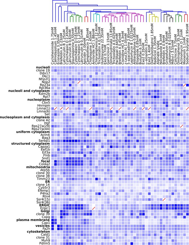
Degree of perturbation for all experimental combinations.
The amount of perturbation for each combination of drug and clone is shown, with deeper shades of blue indicate larger degrees of perturbation (larger distances from the mean feature values for a clone and drug combination to the mean feature values of the vehicle-only control for that clone; feature values are contained in Supplementary file 4). Images were subjected to additional quality control for this analysis; diagonal red lines mark experiments failing this stricter quality control. Clones are grouped by the labels assigned to the unperturbed (control) subcellular localization patterns; the mean perturbation of all proteins with a given label is also displayed for each drug. Drugs were clustered with average linkage using the mean perturbation data. Different tagged variants of the same protein (labeled with clone identifier in parenthesis) sometimes have distinguishably different responses to drugs (e.g. Rps27a clones 29 and 44). Beyond cytotoxic conditions (e.g. Latrunculin B at 1.25 mM) few dominating patterns are apparent; neither unperturbed subcellular compartment nor known targets of drugs are major predictors of the degree of perturbation of most experiments.
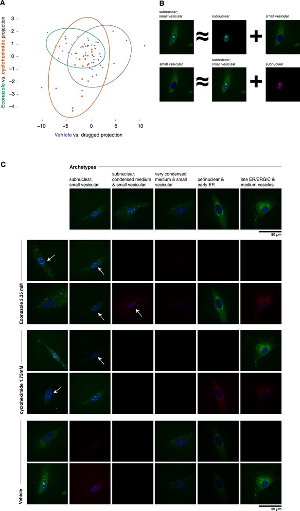
Complex phenotypes arising in top-ranked translocations discovered by the active screen.
EGFP-tagged Fatty acid 2-hydroxylase (Fa2h, clone number 23) expressed in NIH-3T3 cells exhibits a broad range of localization patterns in two top-ranked treatments, cycloheximide (drug 4), and Econazole (drug 16). (A) Image features calculated from confocal images (60X) of two treatments (orange squares and green triangles, respectively) as well as the vehicle treatment (purple dots) are reasonably well classified by logistic regression. The resulting 2D projection of the 173-dimensional feature space transforms the distribution of each treatment into a 2D Gaussian (95% confidence intervals as colored ellipses). Consistent with the active screen results, drug treatments are distinguishable from vehicle and from each other. Fa2h exhibits an unusual spread of secretory-associated, or subnuclear (but not nucleolar), and sometimes both localizations in single cells. (B) In order to visually assess the distributional differences between treatments, we can extend the usual visual vocabulary of coarse localization phenotypes (e.g. 'Golgi,' 'ER' and the like) by decomposing the feature vectors of each single-cell image in terms of a fixed set of single-cell images. Each image can be expressed as an additive combination; for example, a cell exhibiting both a subnuclear and small vesicular localization can be linearly approximated by adding together feature vectors of a subnuclear and a separate small vesicular cell. Subtractive cases (B, bottom row) are false colored with red instead of green for EGFP signal. (C) Archetypal cells (top row), chosen by minimax clustering (Bien and Tibshirani, 2011), can be approximately added in different weighted combinations to reveal nuanced differences in condition-dependent localization (see Materials and methods). For each treatment (pair of rows), two cells (leftmost column) and their additive description in terms of the archetypes are displayed. White arrows highlight dim subnuclear signal where visually subtle. Overall, Econazole appears to have the effect of generally enhancing post perinuclear/ER secretory structure localization, whereas cycloheximide generally suppresses ER localization in favor of presumably later secretory vesicular localization.
Videos
Experiment selection and accuracy of predictions during the active learning process.
Each drug and clone were duplicated in a manner hidden to the active learner (96 x 96 experiments) and are grouped for display purposes together (as 48 x 48). These four biological replicates (which we call a “quad”) are outlined in black, and each is shown separately as a sub-box (not outlined) in its quad. The first frame shows the starting point: unperturbed experiments were measured for all clones (white boxes in a single subcolumn for drug 48) and the model predicted that all drugs lead to the same phenotypes. Each model’s classification accuracy on unseen data is displayed for each 96 x 96 experiment (sub-boxes) in green when correct, and purple when not. For example, the first frame shows that the phenotypes for most drug treatments differed from their corresponding unperturbed condition, and so the overall accuracy was low (more purple than green). By design, the active learner chose the second batch of experiments to evenly sample each drug and clone (sparse white boxes). Those data led to a model with lower accuracy because emphasis was placed on ultimately spurious correlations in phenotypes. In general, the active learner always chose to perform experiments to test presumed correlations in phenotypes, and so there was a substantial increase in accuracy from round 2 to round 3. As additional rounds were performed, the accuracy gradually increased and most quads were only measured once. By round 20, many of the experiments had been correctly predicted and the learner focused on learning the remaining ones. By the last round, most predictions were correct, but the predictions for a few drugs remained largely incorrect.
Tables
Compounds used.
| Compound # | Compound | Stock concentration (mM) (in 100% DMSO) |
|---|---|---|
| 1 | Apicidin | 2.00 |
| 2 | Cytochalasin D | 2.45 |
| 3 | Latrunculin B | 1.25 |
| 4 | Cycloheximide | 1.75 |
| 5 | α-amanitin | 0.25 |
| 6 | Camptothecin | 2.85 |
| 7 | Chloramphenicol | 12.4 |
| 8 | Nocodazole | 8.3 |
| 9 | Diethylstilbestrol | 1.85 |
| 10 | Dinitrophenol | 35.3 |
| 11 | Griseofulvin | 4.95 |
| 12 | Amiloride hcl | 1.88 |
| 13 | Alsterpaullone | 0.85 |
| 14 | Dimenhydrinate | 13.85 |
| 15 | Colchicine | 3.75 |
| 16 | Econazole | 3.35 |
| 17 | Chloroquine | 1.45 |
| 18 | Bulsulfan | 6.1 |
| 19 | Actinomycin D | 1.2 |
| 20 | Radicicol | 1.35 |
| 21 | Calmidazolium | 1.45 |
| 22 | Etoposide | 0.85 |
| 23 | z-Leu(3)-Al | 1.05 |
| 24 | Exo2 | 1.4 |
| 25 | Exo2 | 0.7 |
| 26 | Exo2 | 0.35 |
| 27 | Brefeldin A | 0.9 |
| 28 | Brefeldin A | 0.45 |
| 29 | Brefeldin A | 0.23 |
| 30 | Cytochalasin D | 1.23 |
| 31 | Cytochalasin D | 0.61 |
| 32 | Latrunculin B | 0.63 |
| 33 | Latrunculin B | 0.31 |
| 34 | Staurosporine | 0.55 |
| 35 | Leptomycin B | 0.025 |
| 36 | Trichostatin A | 0.025 |
| 37 | Paclitaxel | 0.645 |
| 38 | Ganciclovir | 3.15 |
| 39 | Monensin | 1.1 |
| 40 | 5-azacytadine | 2.85 |
| 41 | Na butyrate | 2.95 |
| 42 | Hydroxyurea | 22.35 |
| 43 | Clonidine hcl | 4.3 |
| 44 | Alginate lysate | N/A * |
| 45 | Leptomycin B | 1.0125 |
| 46 | Trichostatin A | 0.125 |
| 47 | mdivi-I | 3.55 |
| 48 | Vehicle (No Drug) | N/A |
-
1.3 µL of a given stock were added to 1000 µL, so the final concentrations used are 1/1000 of the concentration listed.
-
* 2.2 mg of the lysate (from Flavobacterium multivorum, Sigma-Aldrich) was dissolved in 2.0 mL DMSO to form the stock solution; units indeterminate.
Additional files
-
Supplementary file 1
This spreadsheet contains the RandTag clone names, tagged gene and subcellular location annotations for the clones used in this work.
- https://doi.org/10.7554/eLife.10047.011
-
Supplementary file 2
The spreadsheet contains the average feature values for all measured experiments, the round each was measured, and the cluster number they were assigned to in each round.
- https://doi.org/10.7554/eLife.10047.012
-
Supplementary file 3
The spreadsheet contains the subcellular pattern labels assigned to each group of phenotypes in Figure 4.
- https://doi.org/10.7554/eLife.10047.013
-
Supplementary file 4
The spreadsheet contains the average feature values for the images for all experiments that passed the post-hoc image quality filtering process, the class each clone was assigned to by visual inspection (for the unperturbed condition), and the distance values that give rise to Figure 5.
- https://doi.org/10.7554/eLife.10047.014


