The geometry and dimensionality of brain-wide activity
- School of Data Science, University of Science and Technology of China, China
- Division of Life Science, The Hong Kong University of Science and Technology, China
- Hefei National Laboratory for Physical Sciences at the Microscale, Center for Integrative Imaging, University of Science and Technology of China, China
- Division of Life Sciences and Medicine, University of Science and Technology of China, China
- Department of Precision Machinery and Precision Instrumentation, University of Science and Technology of China, China
- Department of Mathematics, The Hong Kong University of Science and Technology, China
Figures
Figure 1
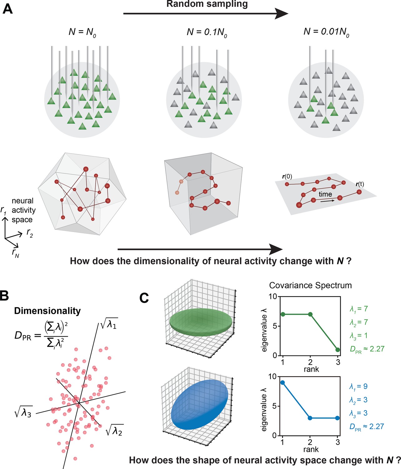
The relationship between the geometric properties of the neural activity space and the size of neural assemblies.
(A) Illustration of how dimensionality of neural activity () changes with the number of recorded neurons. (B) The eigenvalues of the neural covariance matrix dictate the geometrical configuration of the neural activity space with being the distribution width along a principal axis. (C) Examples of two neural populations with identical dimensionality () but different spatial configurations, as revealed by the eigenvalue spectrum (green: , blue: ).
Figure 2 with 4 supplements
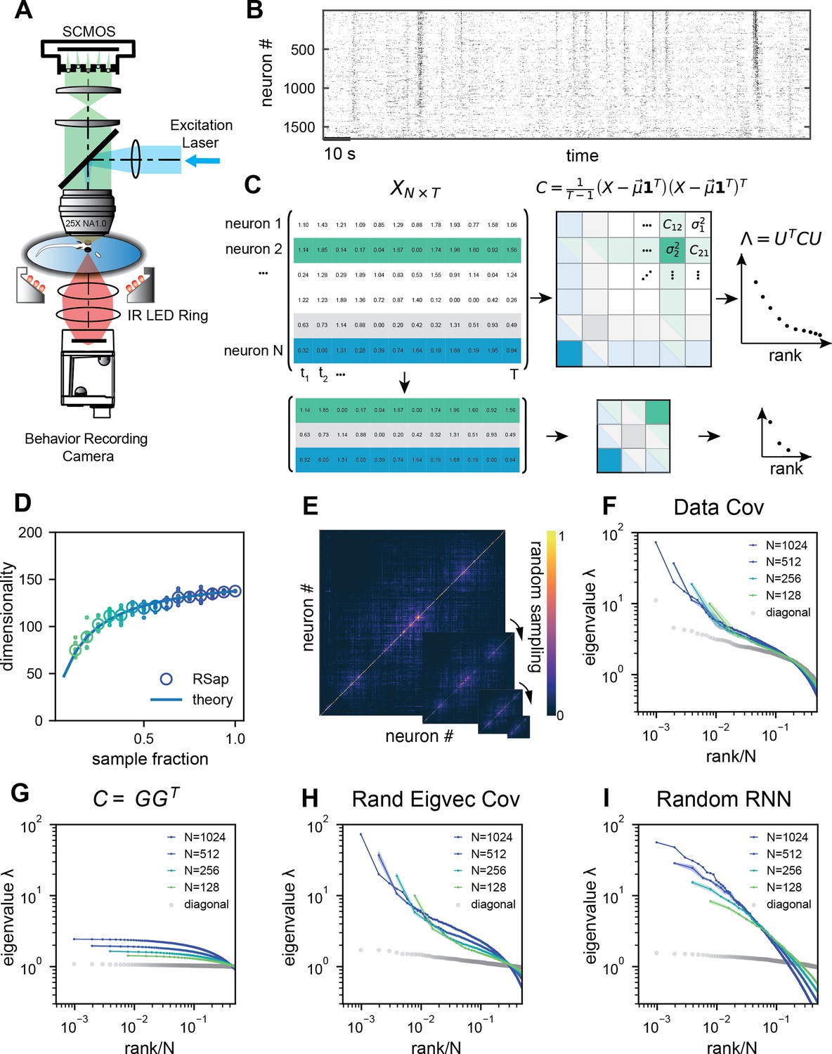
Whole-brain calcium imaging of zebrafish neural activity and the phenomenon of its scale-invariant covariance eigenspectrum.
(A) Rapid light-field Ca2+ imaging system for whole-brain neural activity in larval zebrafish. (B) Inferred firing rate activity from the brain-wide calcium imaging. The ROIs are sorted by their weights in the first principal component (Stringer et al., 2019b). (C) Procedure of calculating the covariance spectrum on the full and sampled neural activity matrices. (D) Dimensionality (circles, average across eight samplings (dots)), as a function of the sampling fraction. The curve is the predicted dimensionality using Equation 5. (E) Iteratively sampled covariance matrices. Neurons are sorted in each matrix to maximize values near the diagonal. (F) The covariance spectra, that is, eigenvalue versus rank/N, for randomly sampled neurons of different sizes (colors). The gray dots represent the sorted variances of all neurons. (G–I) Same as F but from three models of covariance (see details in Methods): (G) a Wishart random matrix calculated from a random activity matrix of the same size as the experimental data; (H) replacing the eigenvectors by a random orthogonal set; (I) covariance generated from a randomly connected recurrent network. The collapse index (CI), which quantifies the level of scale invariance in the eigenspectrum (see Methods), is: (G) CI = 0.214; (H) CI = 0.222; (I) CI = 0.139.
Figure 2—figure supplement 1
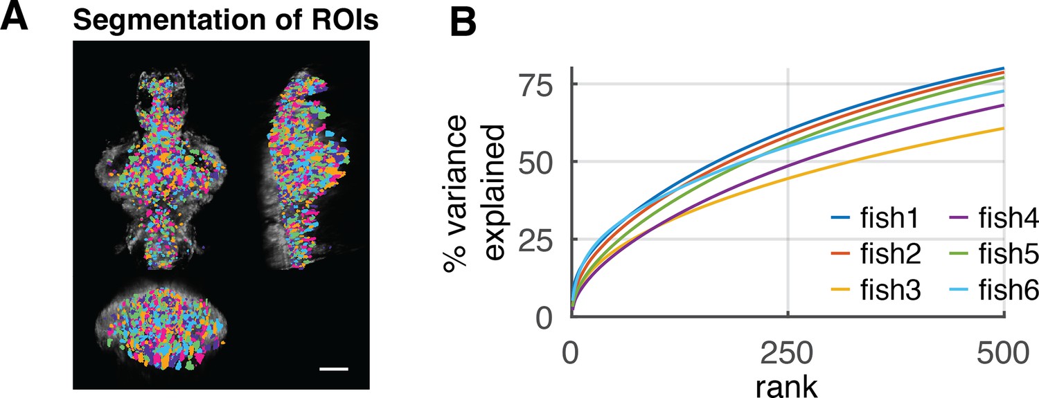
Experimental data description.
(A) Spatial distribution of segmented ROIs (shown in different colors). There are 1347–3086 ROIs in each animal. Scale bar, 100 μm. (B) Explained variance of the activity data by PCs up to 500 rank. The different colored lines represent different fish data (n = 6).
Figure 2—figure supplement 2
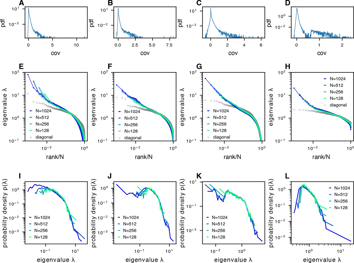
The phenomenon of scale-invariant eigenspectra across different datasets.
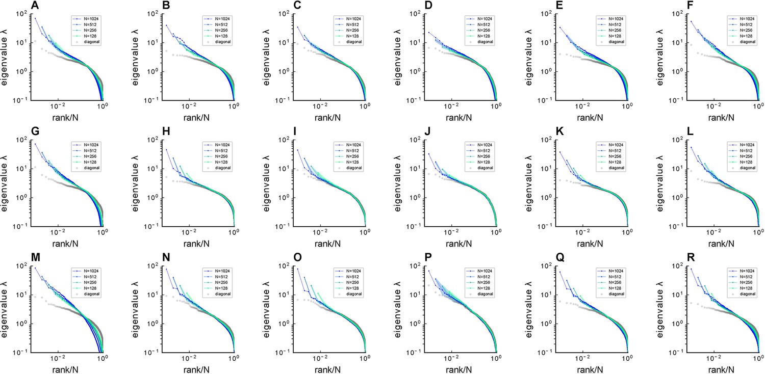
(A–D) Distribution of normalized pairwise covariances, where (Methods). (E–H) Sampled covariance eigenspectra of different datasets. (I–L) Pdfs of sampled covariance matrix eigenspectra of different datasets. The datasets correspond to the following examples: column 1: fish data (from fish 1, all fish data are shown in Figure 5—figure supplement 1A–F) from whole-brain light-field imaging; column 2: fish data from whole-brain light-sheet imaging; column 3: mouse data from multi-area Neuropixels recording; column 4: mouse data from two-photon visual cortex recording.
Figure 2—figure supplement 3
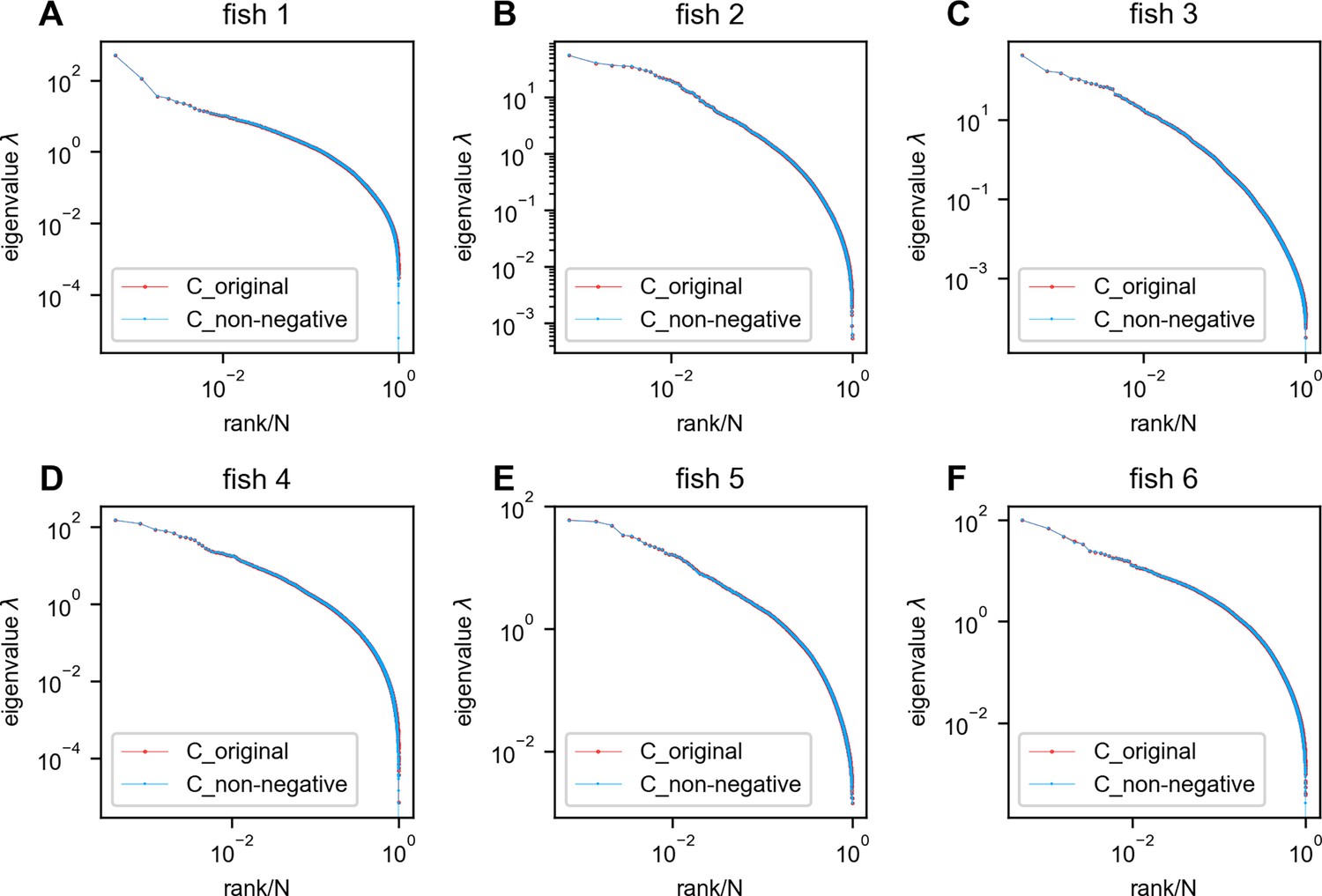
Negative covariances do not affect the eigenspectrum of the zebrafish data.
Red: eigenspectrum of the original data covariance matrix. Blue: eigenspectrum of the covariance matrix with negative entries replaced by zeros. In this figure, all neurons recorded in each fish were utilized without any sampling. (A–F) fish 1 to fish 6.
Figure 2—figure supplement 4
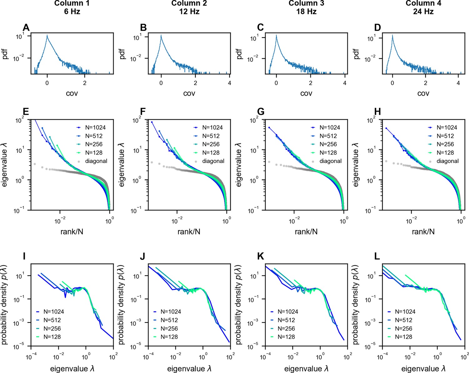
Scale-invariant properties persist across different temporal sampling rates in neural recordings.
Analysis of multi-area Neuropixels recordings (Stringer et al., 2019b) from 1024 neurons, downsampled to different rates resulting in 7200 time frames per condition (6, 12, 18, and 24 Hz; columns 1–4, respectively). (A–D) Distribution of pairwise covariances after normalization to unit variance (, see Methods). (E–H) Eigenvalue spectra of the covariance matrices, showing similar power-law scaling across sampling rates. (I–L) Probability density functions (PDFs) of the eigenvalues, demonstrating that the characteristic shape of the distribution is preserved across different temporal resolutions.
Figure 3 with 2 supplements
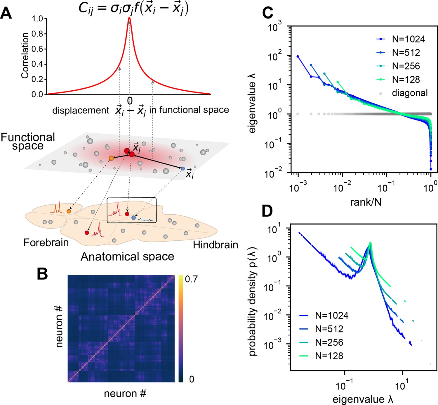
Euclidean Random Matrix (ERM) model of covariance and its eigenspectrum.
(A) Schematic of the ERM model, which reorganizes neurons (circles) from the anatomical space to the functional space (here is a two-dimensional box). The correlation between a pair of neurons decreases with their distance in the functional space according to a kernel function . This correlation is then scaled by neurons’ variance (circle size) to obtain the covariance . (B) An example ERM correlation matrix (i.e., when ). (C) Spectrum (same as Figure 2F) for the ERM correlation matrix in (B). The gray dots represent the sorted variances of all neurons (same as in Figure 2F). (D) Visualizing the distribution of the same ERM eigenvalues in C by plotting the probability density function (pdf).
Figure 3—figure supplement 1
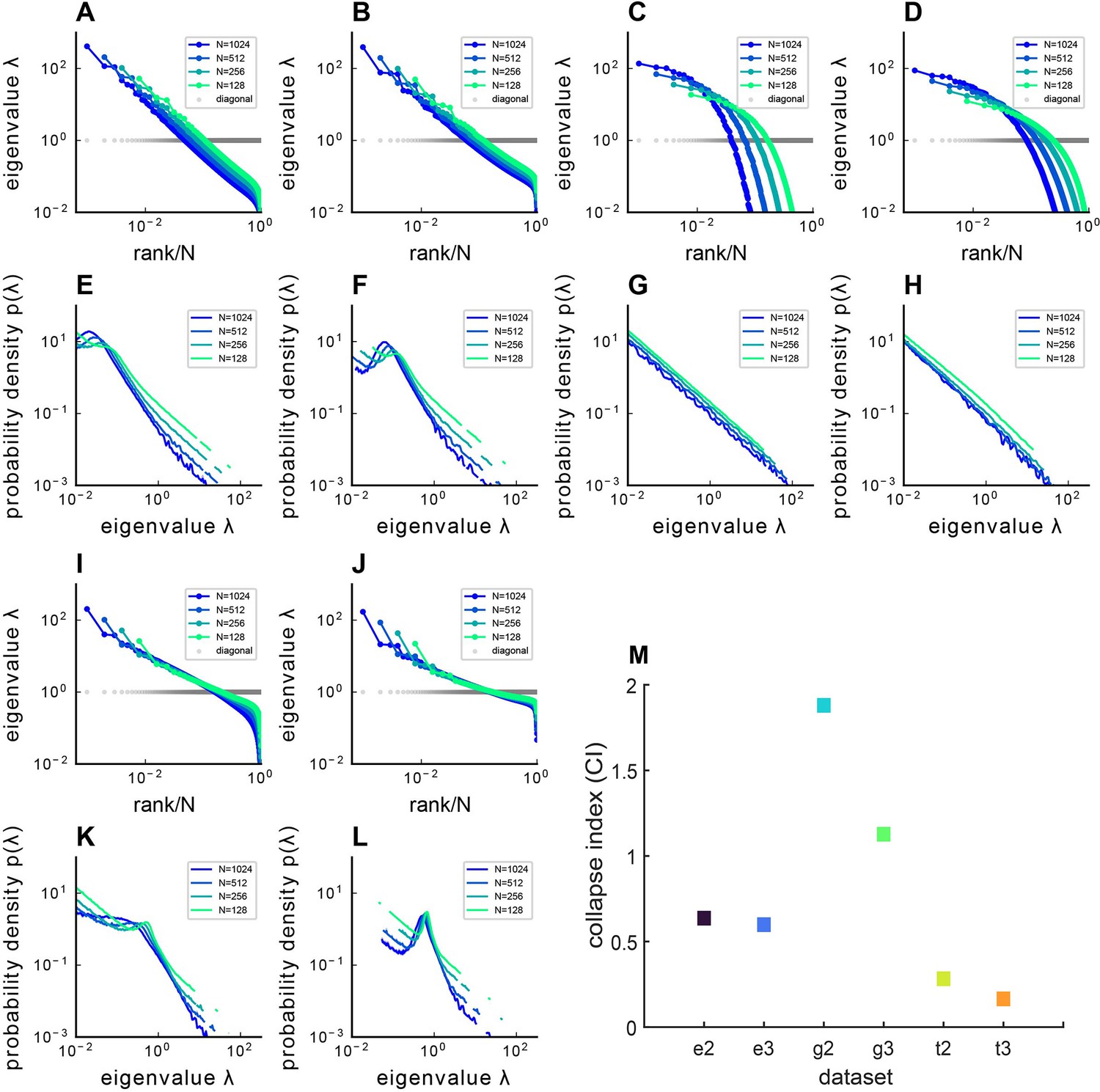
Covariance spectra under different kernel functions .
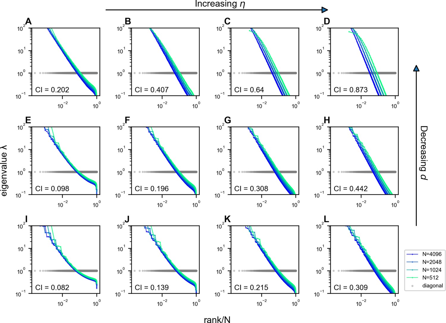
The figure presents both the sampled eigenvalue rank plot and the pdf of Euclidean Random Matrix (ERM) with different functions and varying dimensions , where panels (A–D, I, J) display the rank plot and panels (E–H, K, L) show the pdf of ERM. (A, E) Exponential function where and dimension . (B, F) Exponential function where and dimension . (C, G) Gaussian pdf where and dimension . (D, H) Gaussian pdf where and dimension . (I, K) t pdf (Equation 11) and dimension . (J, L) t pdf (Equation 11) and dimension . The ERM simulations were conducted 100 times and each ERM used an identical sampling technique described in (Methods). The results represent mean ± SEM. (M) Summary of CIs for different and . On the x-axis labels, ‘e’ denotes the Exponential function , ‘g’ denotes the Gaussian pdf , ‘t’ denotes the t-distribution pdf , while ‘2’ and ‘3’ indicate or , respectively.
Figure 3—figure supplement 2
Impact of and on the scale invariance of covariance eigenspectra in the Euclidean Random Matrix (ERM) with .
The columns from left to right correspond to , and the rows from top to bottom correspond to (Equations 2 and 11). Other ERM simulation parameters: , , , , and . Each panel shows a single ERM realization. For visualization purposes, the views in some panels are truncated since we use the same range for the eigenvalues in all panels.
Figure 4 with 2 supplements
Three factors contributing to scale invariance.
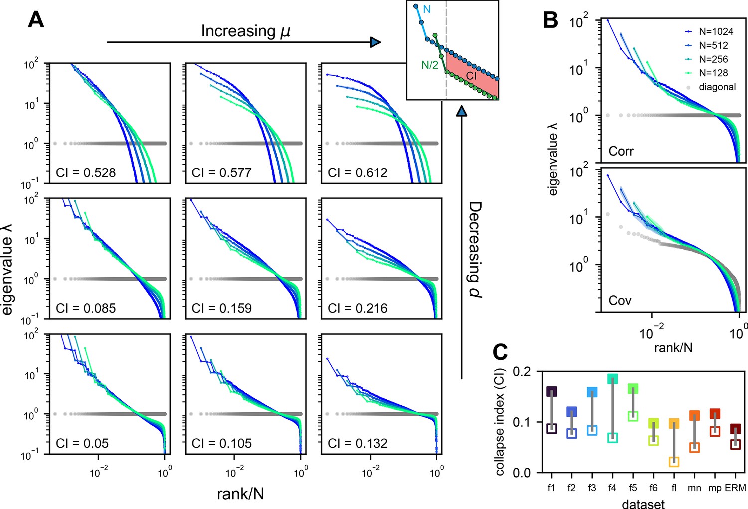
(A) Impact of and (see text) on the scale invariance of Euclidean Random Matrix (ERM) spectrum (same plots as Figure 3C) with . The degree of scale invariance is quantified by the collapse index (CI), which essentially measures the area between different spectrum curves (upper right inset). For comparison, we fix the same coordinate range across panels hence some plots are cropped. The gray dots represent the sorted variances of all neurons (same as in Figure 2F). (B) Top: sampled correlation matrix spectrum in an example animal (fish 1). Bottom: same as top but for the covariance matrix that incorporates heterogeneous variances. The gray dots represent the sorted variances of all neurons (same as in Figure 2F). (C) The CI of the correlation matrix (filled squares) is found to be larger than that for the covariance matrix (opened squares) across different datasets: f1 to f6: six light-field zebrafish data (10 Hz per volume, this paper); fl: light-sheet zebrafish data (2 Hz per volume, Chen et al., 2018); mn: mouse Neuropixels data (downsampled to 10 Hz per volume); mp: mouse two-photon data (3 Hz per volume, Stringer et al., 2019b).
Figure 4—figure supplement 1
Comparison between Euclidean Random Matrix (ERM) simulation and theory.
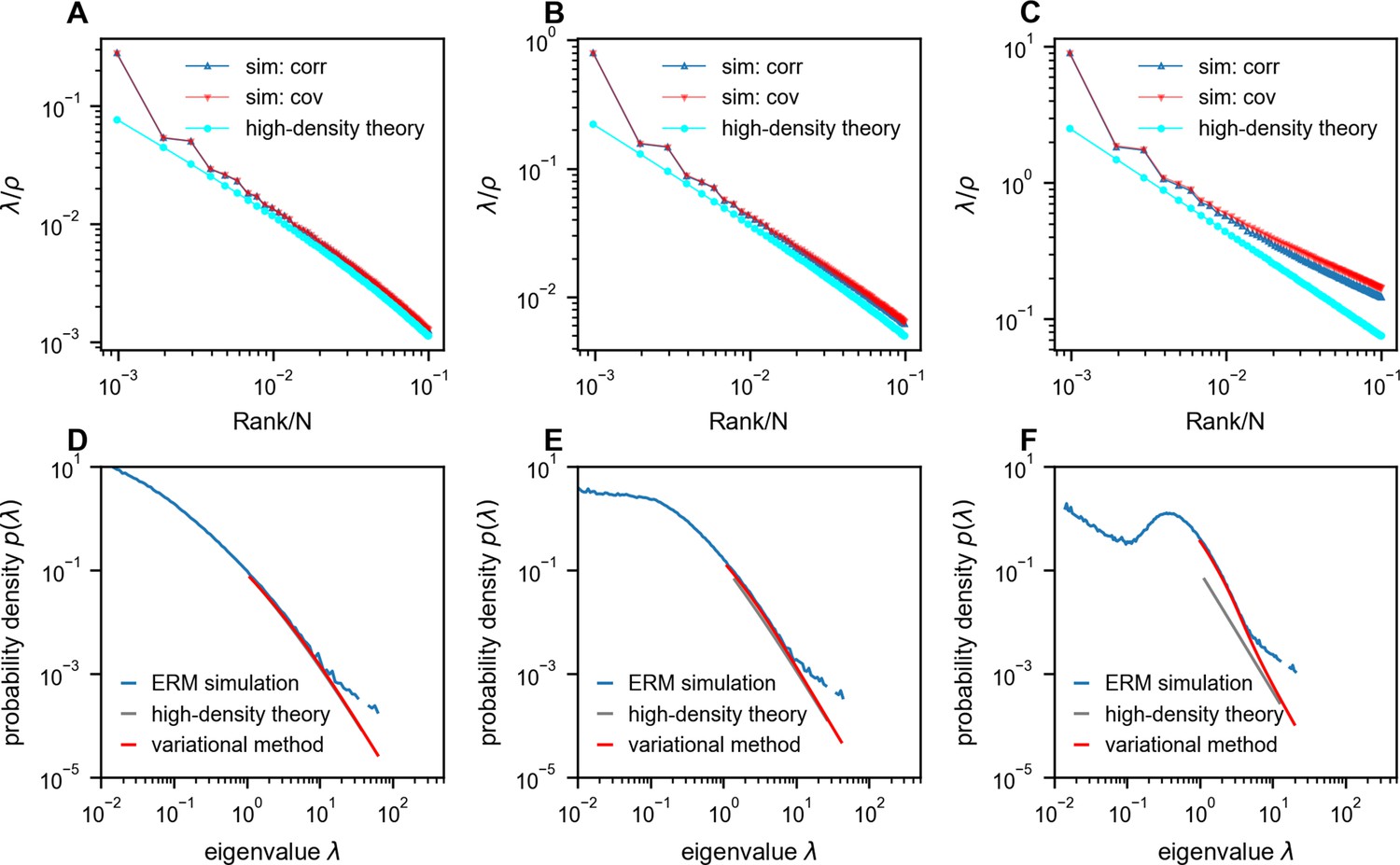
(A–C) Rank plots of the normalized eigenspectra (), with the simulations obtained using correlation matrix (sim: corr, ) and covariance matrix (sim: cov, neuron’s activity variance is i.i.d. sampled from a log-normal distribution with zero mean and a standard deviation of 0.5 in the natural logarithm of the values; we also normalize (Methods)). The curves between ‘sim: corr’ and ‘sim: cov’ are nearly identical in panels (A) and (B). The theoretical predictions of normalized eigenvalues are obtained using the high-density theory (cyan, Equation 12). The density ρ decreases from panel (A) to panel (C) (, respectively). (D–F) Numerical validation of the theoretical spectrum by comparing probability density functions for increasing density of covariance ERM (, respectively). Other simulation parameters: , , , , . The ERM simulations were conducted 100 times. The results are presented as the mean ± SEM.
Figure 4—figure supplement 2
Impact of heterogeneous activity levels on the scale invariance.
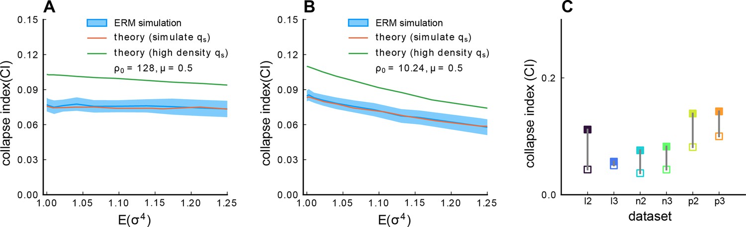
(A) The CI as a function of the heterogeneity of neural activity levels . We generate Euclidean Random Matrix (ERM) where each neuron’s activity variance is i.i.d. sampled from a log-normal distribution where the logarithm of the variable follows a normal distribution with zero mean and a sequence of standard deviation () in the natural logarithm of the values . We also normalize (Methods). The solid blue line is the average across 100 ERM simulations, and the shaded area represents the SD. The red line results from the Gaussian variational method with simulation value integration limit . The green line is the result of the Gaussian variational method with high-density value integration limit (Methods). . (B) Same as A, but with a smaller . Other parameters: , , , , . (C) The collapse index (CI) of the correlation matrix (filled symbols) is larger than that of the covariance matrix (opened symbols) across different datasets excluding those shown in Figure 4. We use 7200 time frame data across all the datasets. l2 to l3: light-sheet zebrafish data (2 Hz per volume); n2 to n3: Neuropixels mouse data, downsampled to 10 Hz per volume, p2 to p3: two-photon mouse data (3 Hz per volume).
Figure 5 with 7 supplements
The relationship between the functional and anatomical space and theoretical predictions.
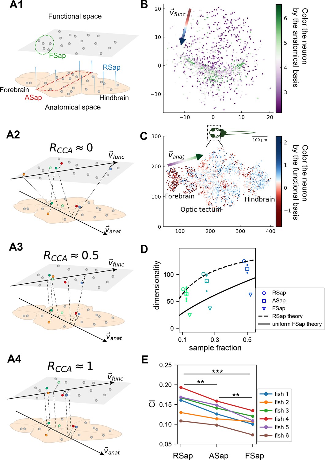
(A) Three sampling methods (A1) and (see text). When (A2), the anatomical sampling (ASap) resembles the random sampling (RSap), and while when (A4), ASap is similar to the functional sampling (FSap). (B) Distribution of neurons in the functional space inferred by MDS. Each neuron is color-coded by its projection along the first canonical direction in the anatomical space (see text). Data based on fish 6, same for (C-E). (C) Similar to (B) but plotting neurons in the anatomical space with color based on their projection along in the functional space (see text). (D) Dimensionality () across sampling methods: average under RSap (circles), average and individual brain region under ASap (squares and dots), and under FSap for the most correlated neuron cluster (triangles; Methods). Dashed and solid lines are theoretical predictions for under RSap and FSap, respectively (Methods). (E) The CI of correlation matrices under three sampling methods in six animals (colors). **p < 0.01; ***p < 0.001; one-sided paired t tests: RSap versus ASap, p = 0.0010; RSap versus FSap, p = 0.0004; ASap versus FSap, p = 0.0014.
Figure 5—figure supplement 1
Fitting Euclidean Random Matrix (ERM) to zebrafish data from our experiments (part 1).
Comparison of sampled covariance eigenspectra in fish data and fitted ERM models. The columns correspond to six light-field zebrafish data: fish 1 to fish 6. Number of time frames: fish 1 – 7495, fish 2 – 9774, fish 3 – 13,904, fish 4 – 7318, fish 5 – 7200, and fish 6 – 9388. (A–F) sampled covariance eigenspectra for different fish data. (G–L) Same as (A–F) but for ERM models with fitted parameters (, ), functional coordinates inferred using MDS, and the experimental . (M–R) Same as (A–F) but for ERM models with fitted parameters (, ), uniform distributed functional coordinates, and a log-normal distribution of . in fish 1–6.
Figure 5—figure supplement 2
Fitting Euclidean Random Matrix (ERM) to all six zebrafish data from our experiments (part 2).
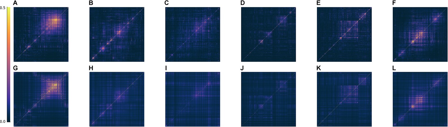
Comparison of the covariance matrix between fish data and our fitted model. The columns correspond to six light-field zebrafish data: fish 1 to fish 6. (A–F) The covariance matrix of different fish data. (G–L) The covariance matrix of ERM models with fitted parameters (, ) and functional coordinates inferred using MDS and the experimental .
Figure 5—figure supplement 3
Fitting Euclidean Random Matrix (ERM) to all six zebrafish data from our experiments (part 3).
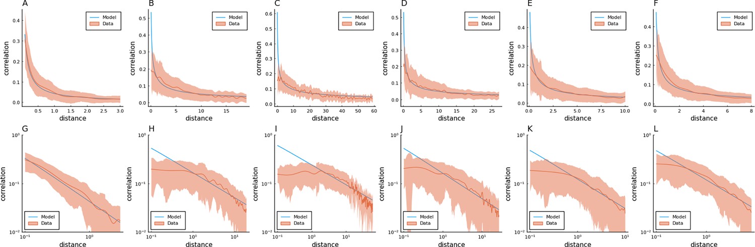
Columns correspond to five light-field zebrafish data: fish 1 to fish 6. (A–F) Comparison of the power-law kernel function in the model (blue line) and the correlation–distance relationship in the data (red line). The distance is calculated from the inferred coordinates using MDS. The shaded area represents the SD. (G–L) Same as (A–D) but on the log–log scale.
Figure 5—figure supplement 4
Fitting Euclidean Random Matrix (ERM) to all six zebrafish data from our experiments (part 4).
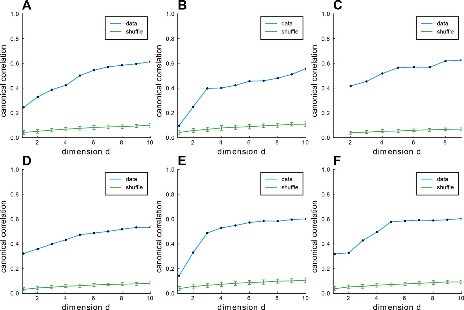
Columns correspond to six light-field zebrafish data: fish 1 to fish 6. (A–F) CCA correlation between the first CCA variables with different embedding dimensions in the functional space. Blue line indicates the CCA correlation of example fish data, green line shows the CCA correlation of example fish data with shuffled functional coordinates, and error bars represent the SD.
Figure 5—figure supplement 5
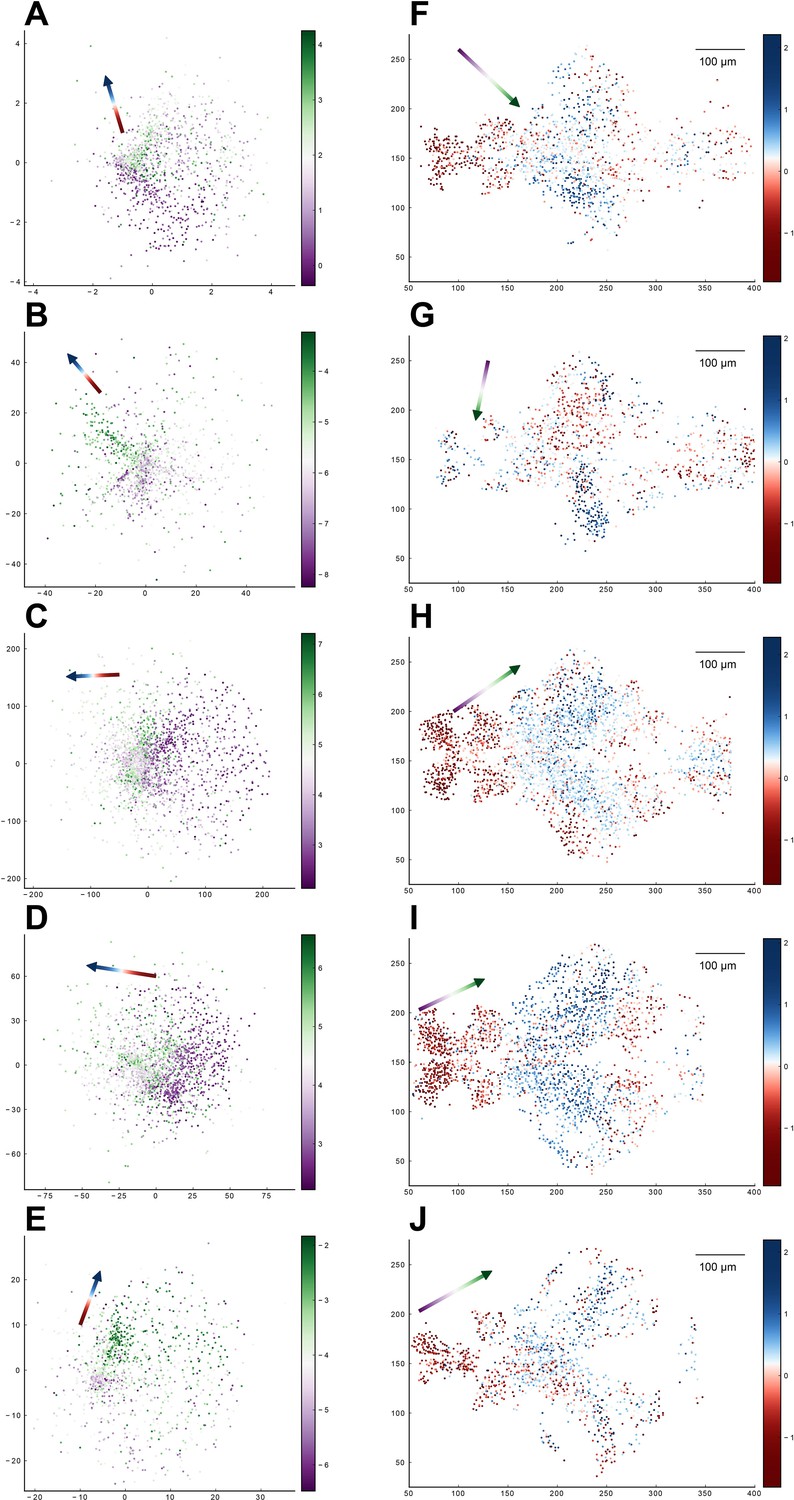
Relationship between the functional space and anatomical space for each zebrafish dataset from our experiments.
Columns correspond to five light-field zebrafish data: fish 1 to fish 5 (with fish 6 has been shown in Figure 5). (A–E) Distribution of neurons in the functional space, where each neuron is color-coded by the projection of its coordinate along the canonical axis in anatomical space (see text in Result). Arrow: the first CCA direction in functional space. (F–J) Distribution of neurons in the anatomical space with the forebrain neuron located on the left side and the hindbrain neuron on the right side. Each neuron is color-coded by the projection of its coordinate along the canonical axis in functional space (see text in Result). Arrow: the first CCA direction in anatomical space.
Figure 5—figure supplement 6
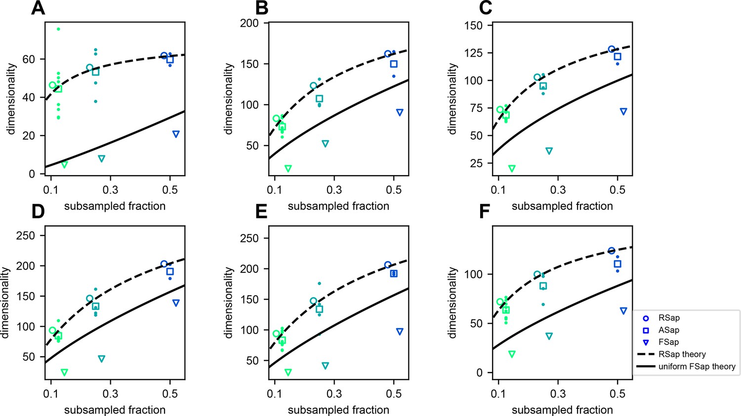
Dimensionality () across sampling methods in fish data.
(A–F) Result from fish 1 to fish 6: mean RSap (circles), mean (squares), and individual ASap , and FSap’s most correlated cluster (triangles). Dashed and solid lines indicate RSap and uniform FSap theoretical predictions, respectively.
Figure 5—figure supplement 7
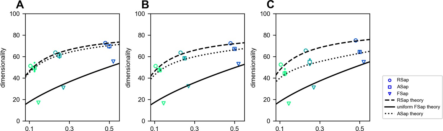
Dimensionality () across sampling methods in Euclidean Random Matrix (ERM).
PR dimensionality result of ERM model, coordinate in funcitonal and anatomical space are multivariate Gaussian distribution, the CCA correlation between funcitonal and anatomical space are in (A–C). Mean RSap (circles), mean (squares), and individual ASap , and FSap’s most correlated cluster (triangles). Dashed and solid lines indicate RSap and uniform FSap theoretical predictions, respectively. ERM parameter: , , functional coordinates follow a multivariate normal distribution with variance , anatomical coordinates follow a multivariate normal distribution with variance .
Appendix 1—figure 1
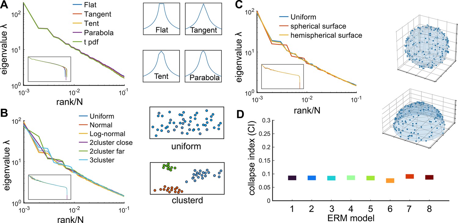
Factors that do not affect the scale invariance.
(A) Rank plot of the covariance eigenspectrum for ERMs with different (see Table 3). Diagrams show different slow-decaying kernel functions along a 1D slice. (B) Same as A but for different coordinate distributions in the functional space (see text). The diagrams on the right illustrate uniform and clustered coordinate distributions. (C) Same as A but for different geometries of the functional space (see text). Diagrams illustrate spherical and hemispherical surfaces. (D) CI of the different ERMs considered in (A–C). The range on the y-axis is identical to Figure 4C. On the x-axis, 1: uniform distribution, 2: normal distribution, 3: log-normal distribution, 4: uniform two nearby clusters, 5: uniform two faraway clusters, 6: uniform 3-cluster, 7: spherical surface in , 8: hemispherical surface in . All ERM models in (B, C) are adjusted to have a similar distribution of pairwise correlations (Appendix 1).
Appendix 1—figure 2
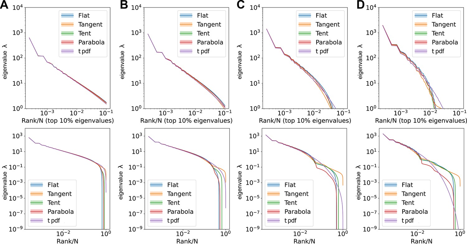
Comparisons of large eigenvalues across different smoothing interval sizes, ε.
Rank plot (upper row) and pdf (lower row) of the covariance eigenspectrum for ERMs with different . (A) . (B) . (C) . (D) . Other ERM simulation parameters: , , , , , . The formulas for different ’s are listed in Table 3 in Methods.
Appendix 1—figure 3
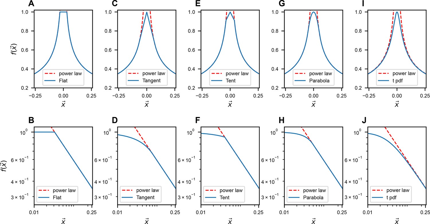
Modifications of near .
The upper row illustrates the slow-decaying kernel function (blue solid line) and its power-law asymptote (red dashed line) along a 1D slice at various . The lower row is similar to A, but on the log–log scale. The formulas for different ’s are listed in Table 3 in Methods.
Appendix 1—figure 4
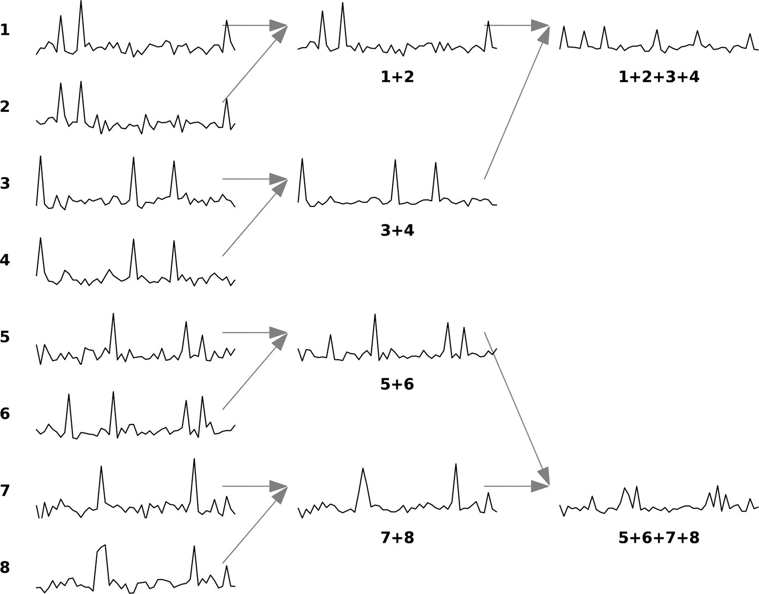
Example of renormalization group (RG) approach for a set of eight neurons.
The figure is adapted from Meshulam et al., 2019. The diagram illustrates the iterative clustering process for eight neurons. In each iteration, neurons are paired based on maximum correlation, with their activities combined through summation and normalized to maintain unit mean for nonzero values. Each neuron can only be paired once per iteration, ensuring all neurons are grouped by the iteration’s end.
Appendix 1—figure 5
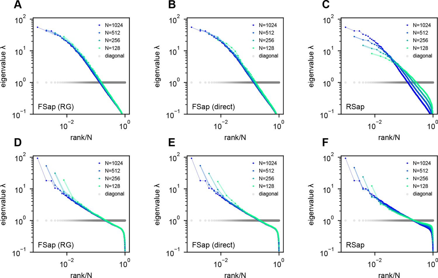
Eigenspectra of renormalization group (RG)-inspired clustering, direct functional region sampling (FSap), and random sampling (RSap) in ERM.
(A, D) RG clustered eigenspectra of ERM. The size of the cluster is denoted by , which is the number of neurons in each cluster. We adopt the RG approach (Meshulam et al., 2018; Meshulam et al., 2019), but with a specific modification (Appendix 1). (B, E) Direct spatial sampling in the functional space (FSap) and the corresponding ERM eigenspectra. We began our analysis with a set of neurons distributed in the functional space. Initially, we chose neurons that were located exclusively on one side of the x-axis of this space. We then proceeded to select neurons from 4 quadrants. This sampling process was repeated iteratively, generating successively smaller subsets of neurons. (C, F) Random sampled (RSap) eigenspectra of ERM. ERM parameters: (A–C) Exponential function where , and dimension . (D–F) Approximate power law Equation 11 with , and dimension . Other parameters are the same as Figure 3. The standard error of the mean (SEM) across the clusters is represented by the shaded area of each line.
Appendix 1—figure 6

Morrell et al.’s latent variable model.
(A–D) Functional sampled (FSap) eigenspectra of the Morrell et al. model. (E–H) Random sampled (RSap) eigenspectra of the same model. Briefly, in Morrell et al.’s latent variable model (Morrell et al., 2024; Morrell et al., 2021), neural activity is driven by latent fields and a place field. The latent fields are modeled as Ornstein–Uhlenbeck processes with a time constant τ. The parameters ε and η control the mean and variance of individual neurons’ firing rates, respectively. The following are the parameter values used. (A, E) Using the same parameters as in Morrell et al., 2021: , , , . Half of the cells are also coupled to the place field. (B–D, F–H) Using parameters from Morrell et al., 2024: , , . There is no place field. The time constant for (B, F, C, G) and (D, H), respectively.
Appendix 1—figure 7
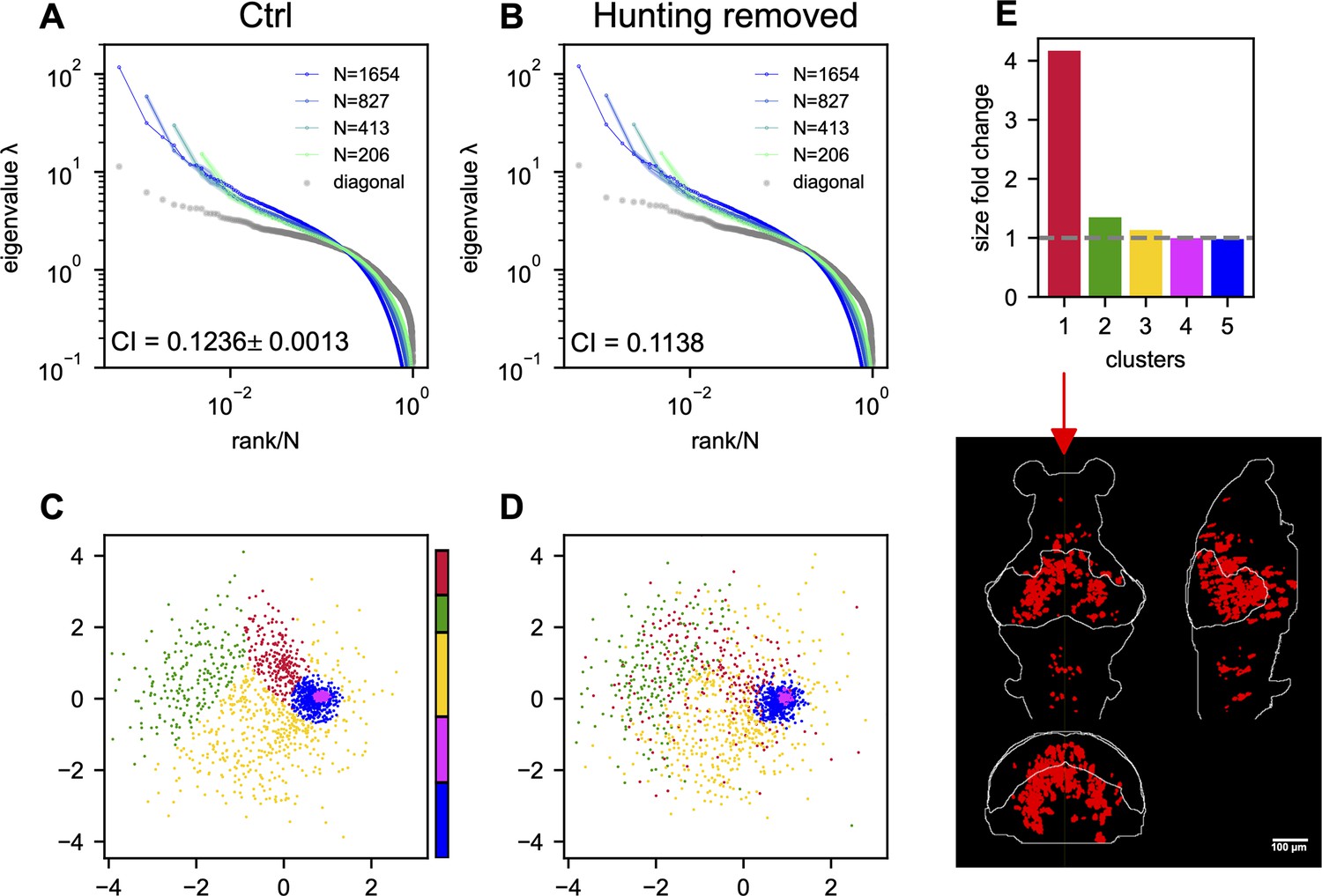
The effects of hunting behavior on scale invariance and functional space organization.
Sampled covariance eigenspectra of the data from fish 1 calculated from control (A) and hunting removed (B) data . Ctrl: We randomly remove the same number of non-hunting frames. This process is repeated 10 times, and the mean ± SD of the CI is shown in the plot. Hunting removed: The time frames corresponding to the eye-converged intervals (putative hunting state) are removed when calculating the covariance (Appendix 1). The CI for the hunting-removed data appears to be statistically smaller than in the control case (p-value = 1.5 × 10⁻⁹). (C) Functional space organization of control data. The neurons are clustered using the Gaussian Mixture Models (GMMs) and their cluster memberships are shown by the color. The color bar represents the proportion of neurons that belong to each cluster. (D) Similar to (C) but the functional coordinates are inferred from the hunting-removed data. The color code of each neuron is the same as that of the control data (C), which allows for a comparison of the changes to the clusters under the hunting-removed condition. See also the Movie S1. (E) Fold change in size/area (Appendix 1) for each cluster (top; the gray dashed line represents a fold change of 1, i.e., no change in size) and the anatomical distribution of the most dispersed cluster (bottom).
Appendix 1—figure 8
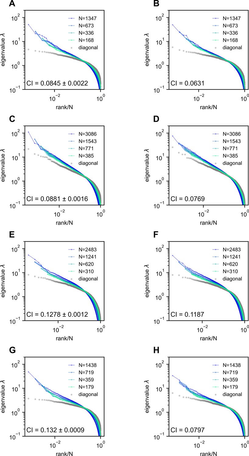
Removing the time segment of hunting behavior does not obliterate the scale-invariant eigenspectra.
Rows correspond to four light-field zebrafish data: fish 2 to fish 5 (results for fish 1 have been shown in Appendix 1—figure 7). (A, C, E, G) Ctrl: we randomly remove the same number of time frames that are not the putative hunting frames. We repeat this process 10 times to generate 10 control covariance matrices and the CI is represented by mean ± SD. (B, D, F, H) Hunting removed: data obtained by removing hunting frames from the full data (Appendix 1). The CI for the hunting removed data appears to be significantly smaller than that of the control case (one-sample t-test in fish 2, in fish 3, in fish 4, and in fish 5).
Appendix 1—figure 9
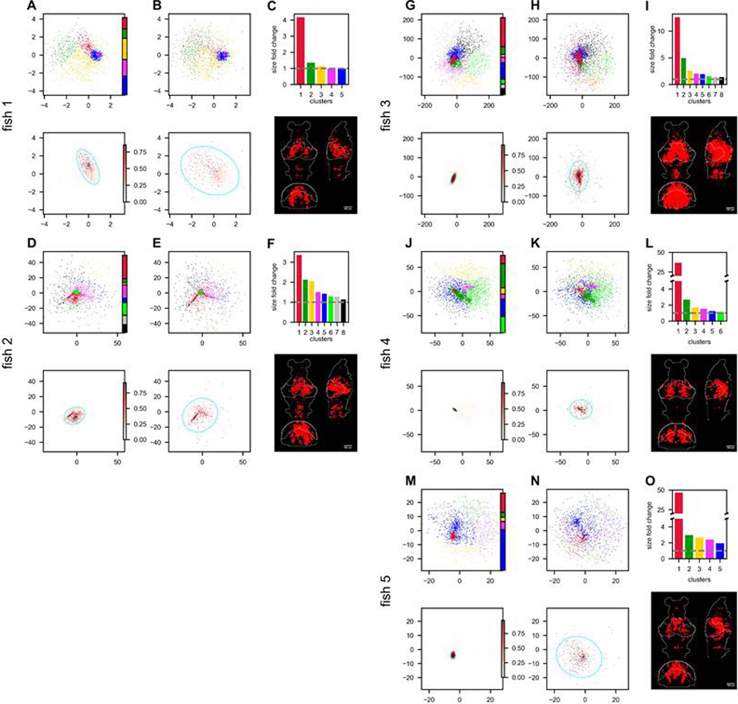
Hunting behavior reorganizes neurons in the functional space (continued on next page).
Rows correspond to five light-field recordings of zebrafish engaged in hunting behavior: fish 1 to fish 5. (A, D, G, J, M) (top) Functional space organization of the control data inferred by fitting the ERM and MDS (Result). Neurons are clustered using the Gaussian Mixture Models (GMMs) and their cluster memberships are shown by the color. The colorbar represents the proportion of neurons belonging to each cluster. (A, D, G, J, M) (bottom) The coordinate distribution of the cluster in control data which is most dispersed (i.e., largest fold change in size, see below) after hunting-removal. The transparency of the dots (colorbar) is proportional to the probability of the neurons belonging to this cluster (Appendix 1). The cyan ellipse serves as a visual aid for the cluster size: it encloses 95% of the neurons belonging to that cluster (Appendix 1). (B, E, H, K, N) (top) Similar to (A, D, G, J, M) (top) but the functional coordinates are inferred from the hunting-removed data. The color code of each neuron is the same as that in the control data, which allows for a comparison of the changes to the clusters under the hunting-removed condition. (B, E, H, K, N) (bottom) Similar to (A, D, G, J, M) (bottom) but the functional coordinates are inferred from the hunting-removed data. The transparency of each neuron is the same as in (A, D, G, J, M). (bottom), and it represents the probability (Appendix 1) of neurons belonging to the most dispersed cluster in the control data. Likewise, the cyan ellipse encloses 95% of the neurons belonging to that cluster (Appendix 1). (C, F, I, L, O) Top, size/area fold change (Appendix 1) for each cluster (the gray dashed line represents a fold change of 1, i.e., no change in size); bottom, the anatomical distribution of the neurons in the most dispersed cluster.
Appendix 2—figure 1
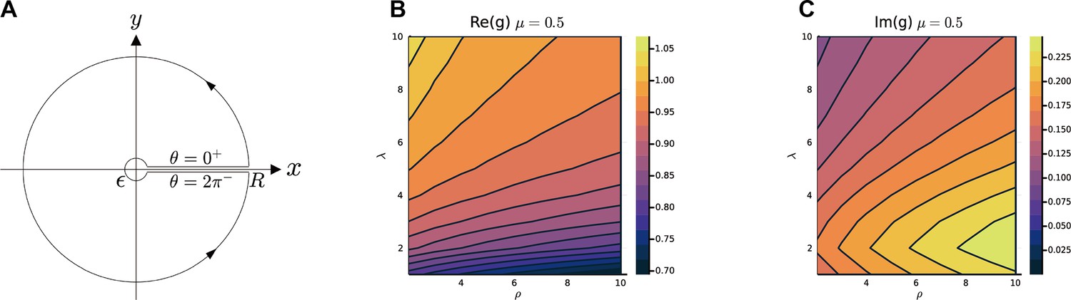
Calculate and .
(A) The path of the contour integral for , (Equation S70). The heatmap of and with respect to λ and ρ, in (B, C) are calculated by the numerical method (Methods). The parameters are , , , , , is i.i.d. sampled from a log-normal distribution with zero mean and a standard deviation of 0.5 in the natural logarithm of the values; we also normalize .
Appendix 2—figure 2
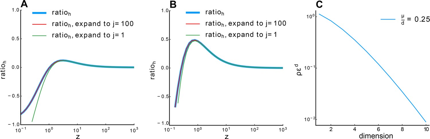
Relationship between and .
(A) , (B) . Blue line: calculated numerically. Red line: 100-order expansion of Equation S104, which perfectly overlaps with the blue line. Green line: expansion to the first order. Other parameter: , , . (C) Relationship between and dimension with fixed Equation S108.
Appendix 2—figure 3
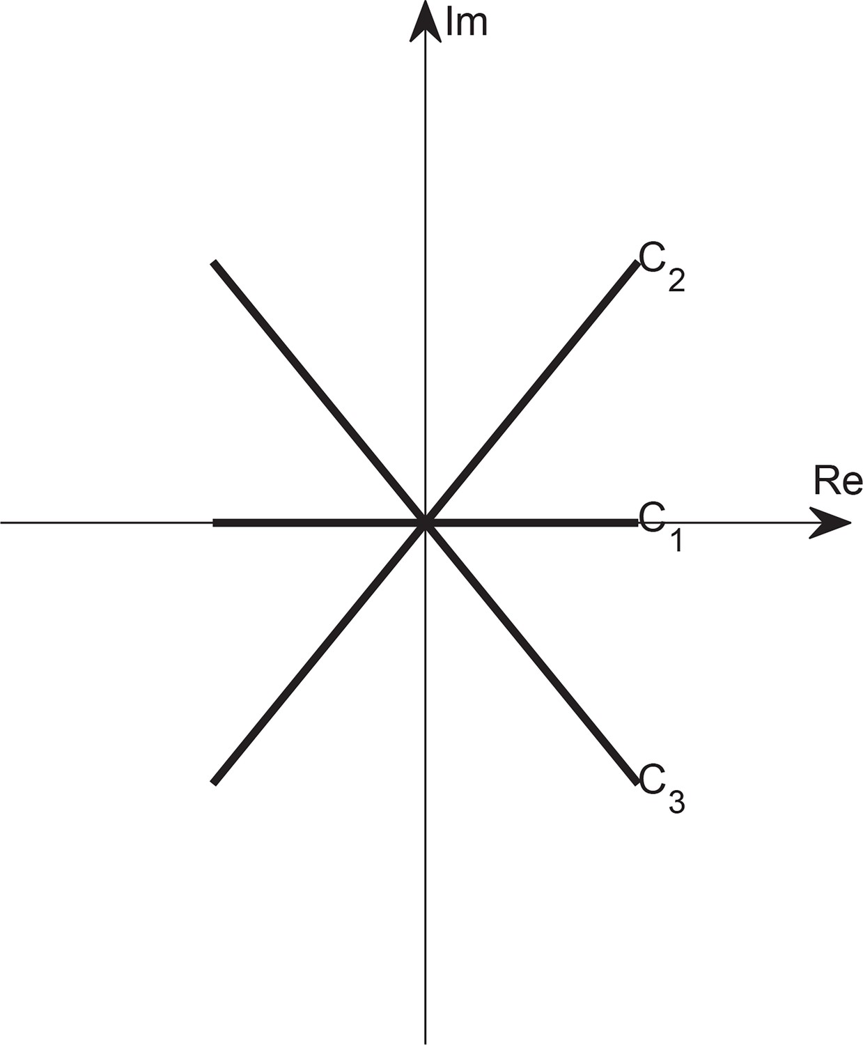
Wick rotation in complex plane.
Author response image 1
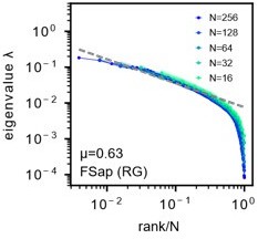
Morrell’s latent model.
A: We reproduce the results as presented in Morrell et al., PRL 126(11), 118302 (2021) [4]. Parameters are same as Fig. S23A. Sampled 16 to 256 neurons. Unlike in our study, the mean eigenvalues are not normalized to one. Dashed line: eigenvalues fitted to a power law. See also Morrell et al. [4] Fig.1C. Parameters are same as Author response image 1. µ is the power law exponent (black) of the fit, which is different from the µ parameter used to characterize the slow decay of the spatial correlation function, but corresponds to the parameter α in our study.
Videos
Appendix 1—video 1
Neural activity patterns in anatomical and functional space during hunting (click here).
Single-trial examples of fish 1 and fish 3. (A) Inferred firing rate activity in anatomical space. Scale bar, 100 µm. (B) Inferred firing rate activity in functional space. Functional space organization of the control data inferred by fitting the ERM and MDS in Result. The cyan ellipse serves as a visual aid for the cluster size: it encloses 95% of the neurons belonging to that cluster (Appendix 1). The inset illustrates the functional space organization, similar to that shown in Appendix 1—figure 7C. The colorbars in panels A and B depict the inferred activity magnitude of individual neurons. (C) Simultaneous behavior recording alongside the neural activity. Time, seconds.
Tables
Table 1
Table of notations.
| Notation | Description |
|---|---|
| Covariance matrix, Equation 2 | |
| Pairwise covariance between neuron i, j; entries of | |
| Participation ratio dimension, Equation 5 | |
| Anatomical sampling dimension, Equation 4 | |
| λ | Eigenvalue of a covariance matrix |
| Probability density function of covariance eigenvalues, Equation 8 | |
| r | Rank of an eigenvalue in descending order, Equation 3 |
| q | Fraction of eigenvalues up to λ and ; Equation 13 |
| Kernel function or distance-correlation function, Equation 11 | |
| Fourier transform of | |
| μ | Power-law exponent in , Equation 11 |
| ε | Resolution parameter in to smooth the singularity near 0, Equation 11 |
| Number of neurons | |
| The total number of neurons prior to sampling | |
| k | the fraction of sampled neurons |
| Linear box size of the functional space | |
| ρ | Density of neurons in the functional space, Equation 3 |
| Dimension of the functional space, Equation 3 | |
| Neural activity of neuron i at time t | |
| Temporal variance of neural activity, Equation 2 | |
| Cl | Collapse index for measuring scale invariance, Equation 13 |
| α | Power-law coefficient of eigenspectrum in the rank plot, see Discussion |
| Neuron i's coordinate in the functional and anatomical space, respectively | |
| The first canonical directions in the functional and anatomical space, respectively | |
| The first canonical correlation | |
| Correlation between anatomical and functional coordinates along ASap direction, Equation 4 |
Key resources table
| Reagent type (species) or resource | Designation | Source or reference | Identifiers | Additional information |
|---|---|---|---|---|
| Strain, strain background (Danio rerio) | Tg(elavl3: H2B- GCaMP6f) | https://doi.org/10.7554/eLife.12741 | Jiu-Lin Du, Institute of Neuroscience, Chinese Academy of Sciences, Shanghai | |
| Software, algorithm | julia1.7 | https://julialang.org/ | ||
| Software, algorithm | MATLAB | https://ww2.mathworks.cn/ | ||
| Software, algorithm | Mathematica | https://www.wolfram.com/mathematica/ |
Table 2
Resources for additional experimental datasets.
| Dataset | Data reference |
|---|---|
| Light-sheet imaging of larval zebrafish (Chen et al., 2018) | https://janelia.figshare.com/articles/dataset/Whole-brain_light-sheet_imaging_data/7272617 |
| Neuropixels recordings in mice (Stringer et al., 2019b) | https://janelia.figshare.com/articles/dataset/Eight-probe_Neuropixels_recordings_during_spontaneous_behaviors/7739750 |
| Two-photon imaging in mice (Stringer et al., 2019b) | https://janelia.figshare.com/articles/dataset/Recordings_of_ten_thousand_neurons_in_visual_cortex_during_spontaneous_behaviors/6163622 |
Table 3
Modifications of the shape of near used in Appendix 1—figures 1–3.
Flat: when , . Tangent: when , follows a tangent line of the exact power law ( and have a same first-order derivative when ). b and c are constants. Tent: when , follows a straight line while the slope is not the same as the tangent case. Parabola: when , follows a quadratic function ( and have same first-order derivative). t pdf: mimic the smoothing treatment like the t distribution. All the constant parameters are set such that .
| Definition | |
|---|---|
| Flat | |
| Tangent | |
| Tent | |
| Parabola | |
| t pdf |
Appendix 2—table 1
Table of notations.
| Notation | Description |
|---|---|
| Resolvent Equation S5 | |
| The average across realizations of 𝐶 (i.e., random and ’s), Equation S4 | |
| Canonical partition function, Gaussian integral representation of the determinant , Equation S8 | |
| Intermediate variable for Gaussian integral representation , Equation S8 | |
| Density field of | |
| Respective Lagrange multiplier fields of | |
| The action in (by analogy with the path integral formulation of quantum mechanics) | |
| The action in the high-density approximation of | |
| The action in the variational approximation of | |
| Term in | |
| The operator inverse of , Equation S26 | |
| Quadratic kernel in the Gaussian integral approximation of | |
| The operator inverse of , same definition as | |
| The Fourier transform of |
Additional files
Download links
A two-part list of links to download the article, or parts of the article, in various formats.
Downloads (link to download the article as PDF)
Open citations (links to open the citations from this article in various online reference manager services)
Cite this article (links to download the citations from this article in formats compatible with various reference manager tools)
The geometry and dimensionality of brain-wide activity
eLife 14:RP100666.
https://doi.org/10.7554/eLife.100666.3


