Untwisting the Caenorhabditis elegans embryo
- National Institutes of Health, United States
- Sloan-Kettering Institute, United States
- Yale University School of Medicine, United States
- Zhejiang University, China
- University of Connecticut Health Center, United States
Figures
Figure 1 with 4 supplements

Key steps in worm untwisting.
(A) An image of a threefold embryo in the twisted state, showing the untwisting markers. (B) The same image as in (A) with the untwisting markers labeled. Asterisks mark seam cell nuclei, and the dashed line indicates the midline marker. (C) The same embryo as in (A, B), after untwisting. Asterisks and dashed line as in B. (D–F) Further detail lattice creation and splines that model embryo. (D) Left: same embryo volume as in (A). Right: accompanying schematic showing the seam cell nuclei in the twisted embryo (black circles) and midline (interior black line). (E) Lattice creation. As diagrammed in right schematic, parts (1) and (2), the user adds points to create a lattice (blue and yellow lines). After the lattice is built, the algorithm generates splines defining the edges of the worm (orange and purple lines) automatically. The midline is also defined with a spline (red line at left). (F) The embryo volume and accompanying schematic showing a completed lattice and model. (G) The embryo volume and accompanying schematic after untwisting. All scale bars: 10 μm.
Figure 1—figure supplement 1
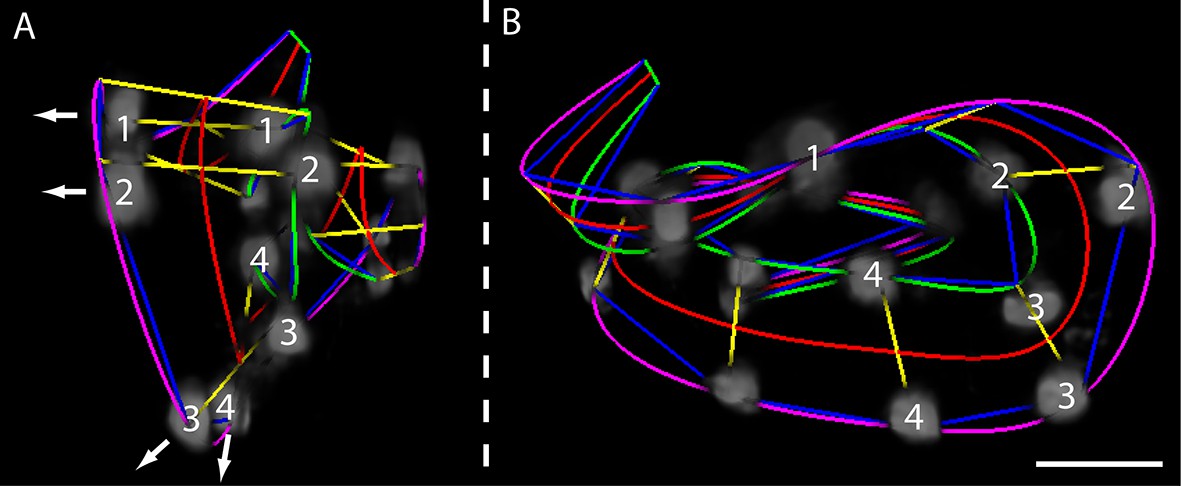
Helical twisting in the nematode embryo.
(A) Evidence for helical twisting, highlighted on four pairs of consecutive seam cell nuclei. If no helical twisting occurs, yellow lines (connecting seam cell nucleus pairs) should appear parallel to each other when sighting down the midline of the worm (red line). If helical twisting is present, yellow lines should appear to twist about the midline. Arrows denote the direction of lines for four pairs of consecutive seam cell nuclei: note obvious and apparent angular twist between pairs 1 and 4. (B) Side view showing same data as in (A). As before, nuclei pairs 1 and 4 appear in close to perpendicular orientation to each other, despite the roughly parallel midline. Scale bar: 10 μm.
Figure 1—figure supplement 2
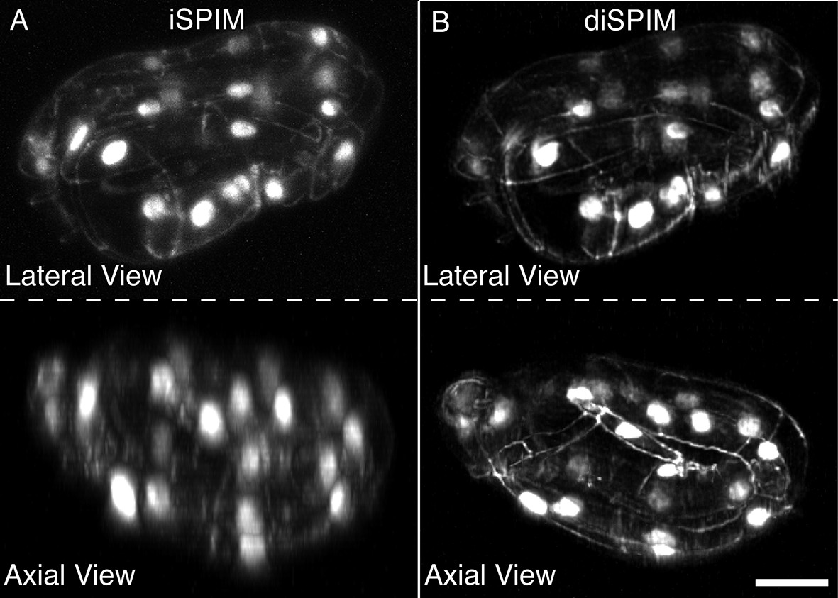
DiSPIM is useful in identifying landmarks in the twisted embryo.
Coarse features such as seam cell nuclei are visible in single view iSPIM (A), but finer features such as junctions between hypodermal cells labeled with DLG-1::GFP are better resolved in the diSPIM (B), particularly in the axial direction (lower row). Scale bar: 10 μm. diSPIM, dual-view Selective Plane Illumination Microscopy; iSPIM, inverted Selective Plane Illumination Microscopy.
Figure 1—figure supplement 3
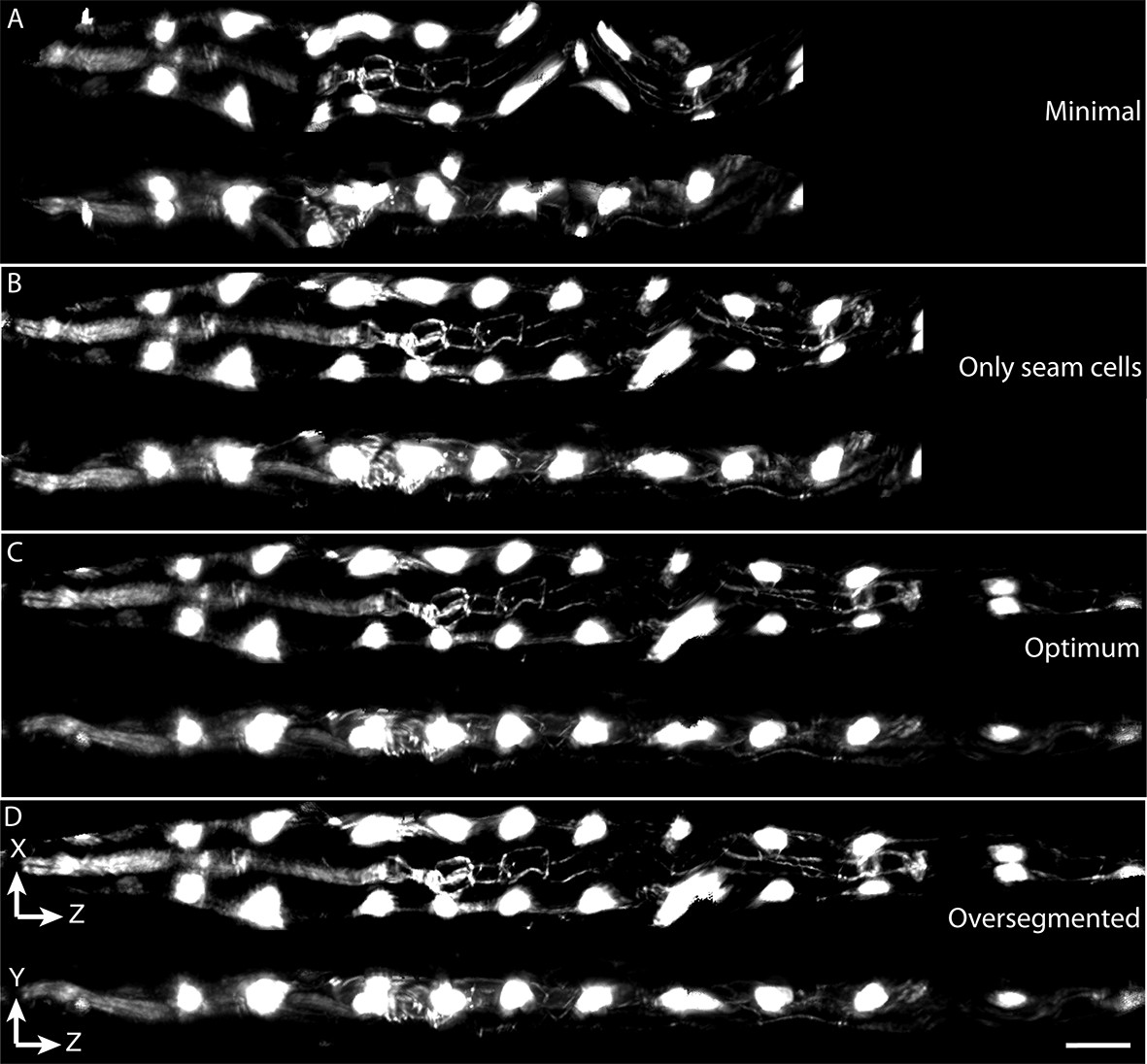
Effects of lattice point number on untwisting results.
(A) XZ and YZ views of an untwisted worm embryo using a lattice comprised of every other seam cell nucleus, a total of 12 points. This lattice fails to capture bends in the animal and does not create smooth left and right edges in the untwisted worm embryo. (B) Same as (A) but using a lattice built with all seam cell nuclei and the nose, a total of 22 points. This lattice still fails to capture some bends in the worm, and the extension of the tail. (C) Same as (A) but using a lattice built with all seam cell nuclei as well as additional points in highly bent regions in the worm embryo, plus a pair of points marking the tail, for a total of 28 points. Bends are accurately captured in the resulting untwisted volume. (D) Several additional lattice points were added to the lattice in (C), along the edges of the animal, for a total of 36 points. No noticeable improvements are apparent. Scale bar: 10 μm.
Figure 1—figure supplement 4
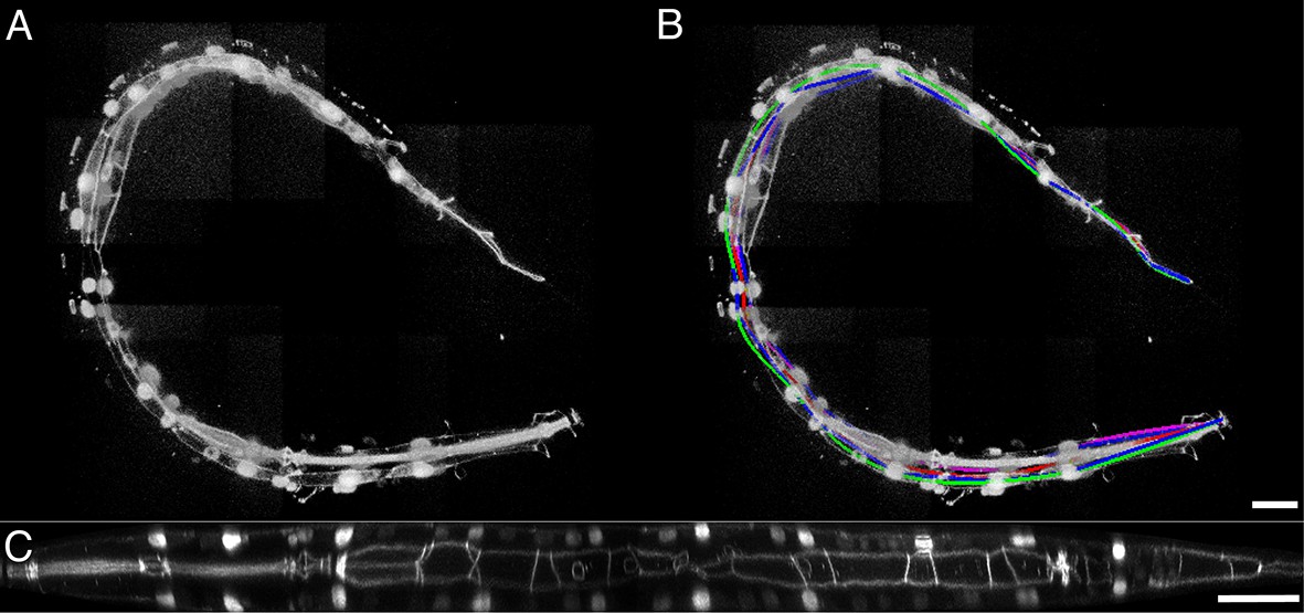
Untwisting a larval nematode.
(A) The twisted L2 larval volume displayed in the MIPAV volume renderer. (B) The twisted L2 larva after lattice-building. (C) The L2 larval worm after untwisting. See also Video 7. MIPAV, Medical Image Processing, Analysis, and Visualization
Figure 2 with 1 supplement
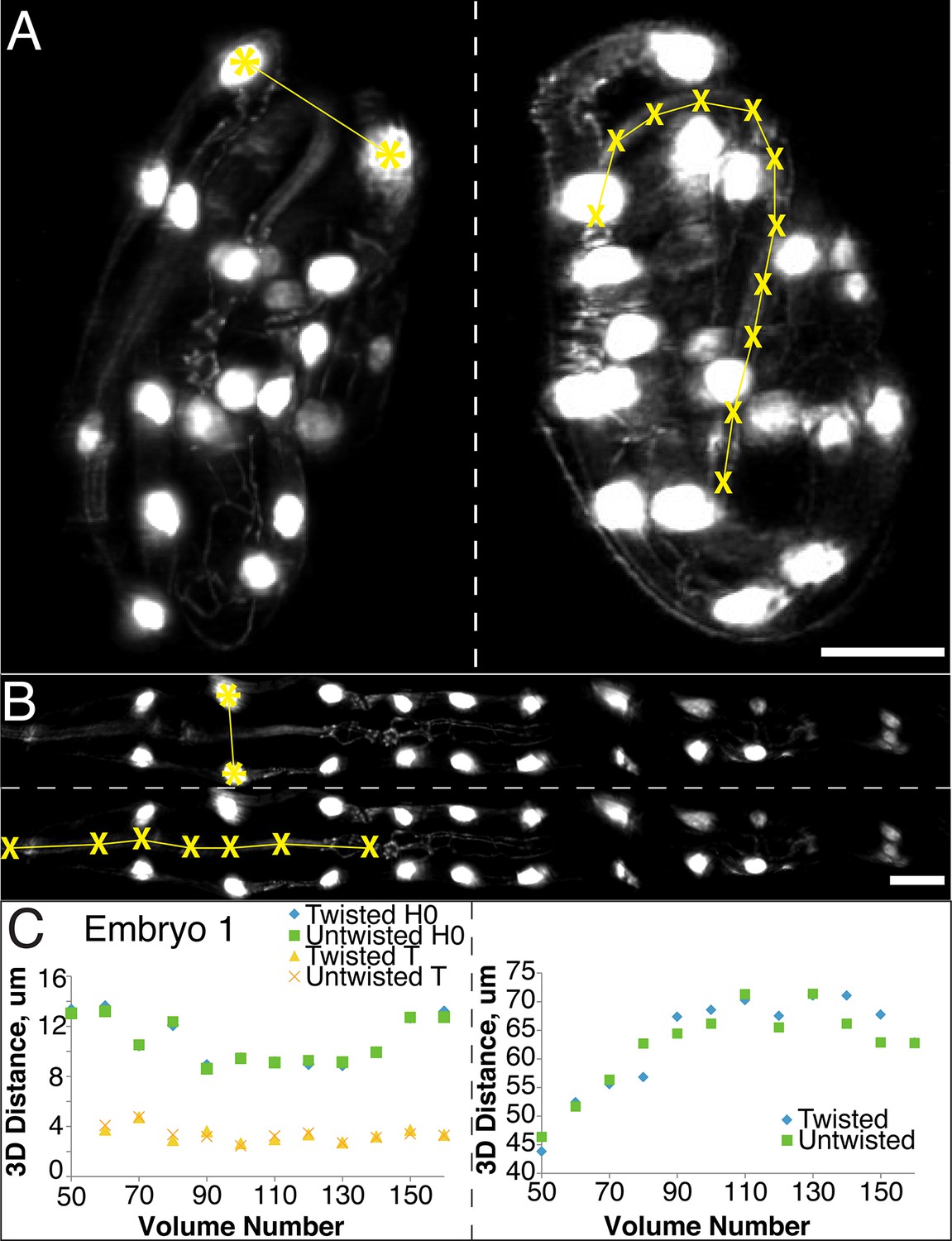
The untwisting algorithm accurately preserves embryo dimensions.
Distances between seam cell nuclei (left) and pharyngeal lengths (right) were compared in twisted (A) and untwisted (B) worm embryos. All scalebars: 10 µm. (C) Comparative 3D distance measurements of seam cell nuclei pairs H0 and T (left graphs) and pharyngeal lengths (right graphs) for one representative embryo (a comparison across six different embryos is presented in Figure 2—figure supplement 1). In all cases, distance measurements in the twisted case are within 5 μm of distance measurements in the untwisted case.
Figure 2—figure supplement 1
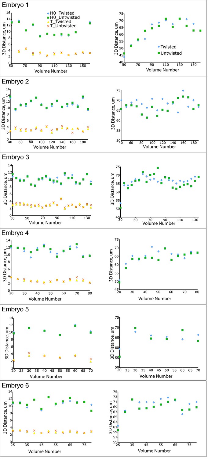
Untwisting does not systematically alter worm morphology
Comparative 3D distance measurements of seam cell nuclei pairs H0 and T (left graphs) and pharyngeal lengths (right graphs) for six embryos. In all cases, distance measurements in the twisted case are within 10 μm of distance measurements in the untwisted case.
Figure 3 with 3 supplements
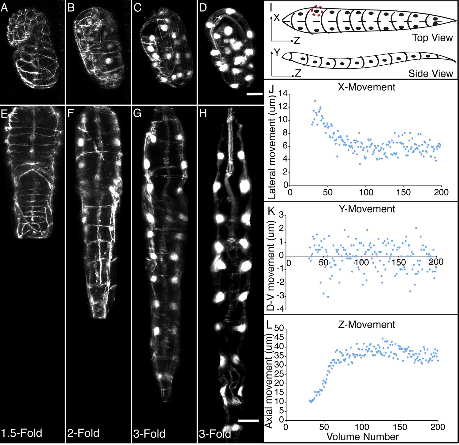
Morphological changes in embryonic development, as unveiled by untwisting algorithm.
Selected volumetric timepoints pre (A–D) and post (E–H) untwisting, with canonical state of embryo indicated at bottom. See also Video 2. (I) Cartoon of untwisted embryo, indicating coordinate system. (J–L) X, Y, and Z movements of circled seam cell nucleus in (I). Measurements are indicated relative to the animal’s nose, fixed as the origin in all untwisted datasets. All scalebars: 10 μm.
Figure 3—figure supplement 1
Comparison of untwisted 1.5-fold embryos after shifting.
Comparative timepoints were selected based on the H1R seam cell shifts. Max projections of volumetric images are shown. Note the underlying similarity in overall shape across animals. Scalebar: 5 μm.
Figure 3—figure supplement 2
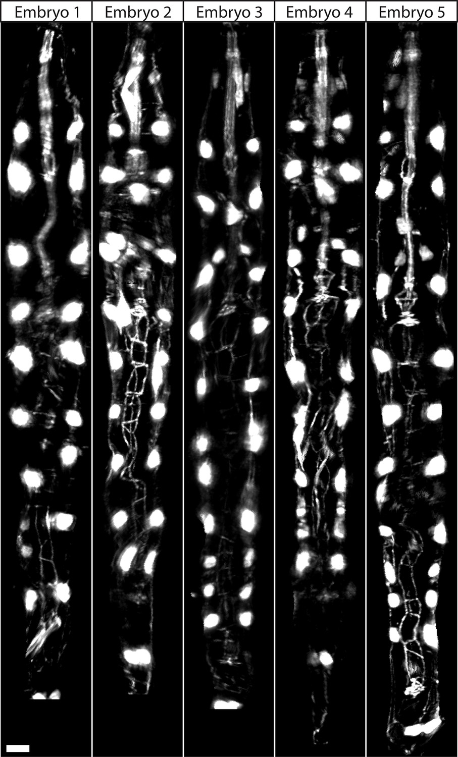
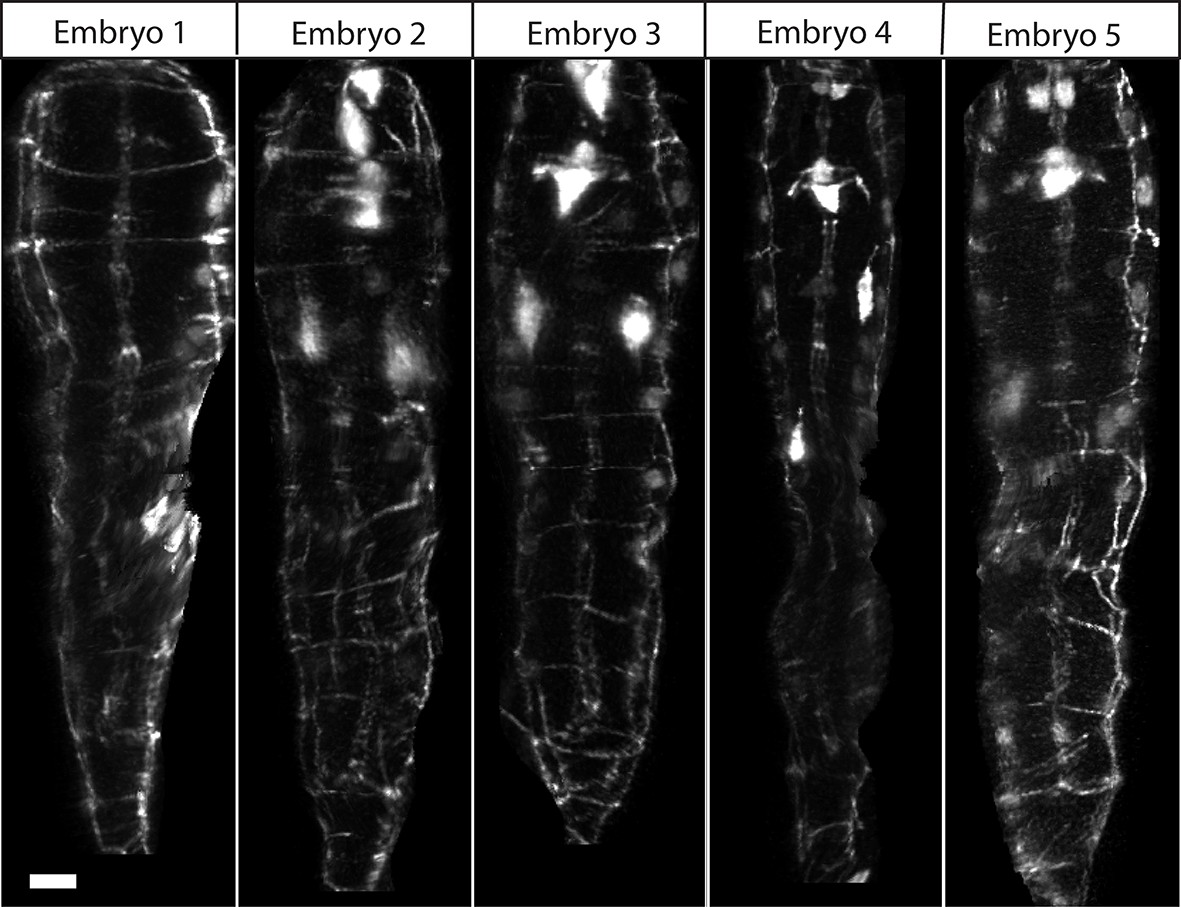
Comparison of threefold embryos after shifting.
Comparative timepoints were selected based on the H1R seam cell shifts. Max projections of volumetric images are shown. Note the underlying similarity in overall shape and seam cell positions across animals. Scalebar: 5 μm.
Figure 3—figure supplement 3
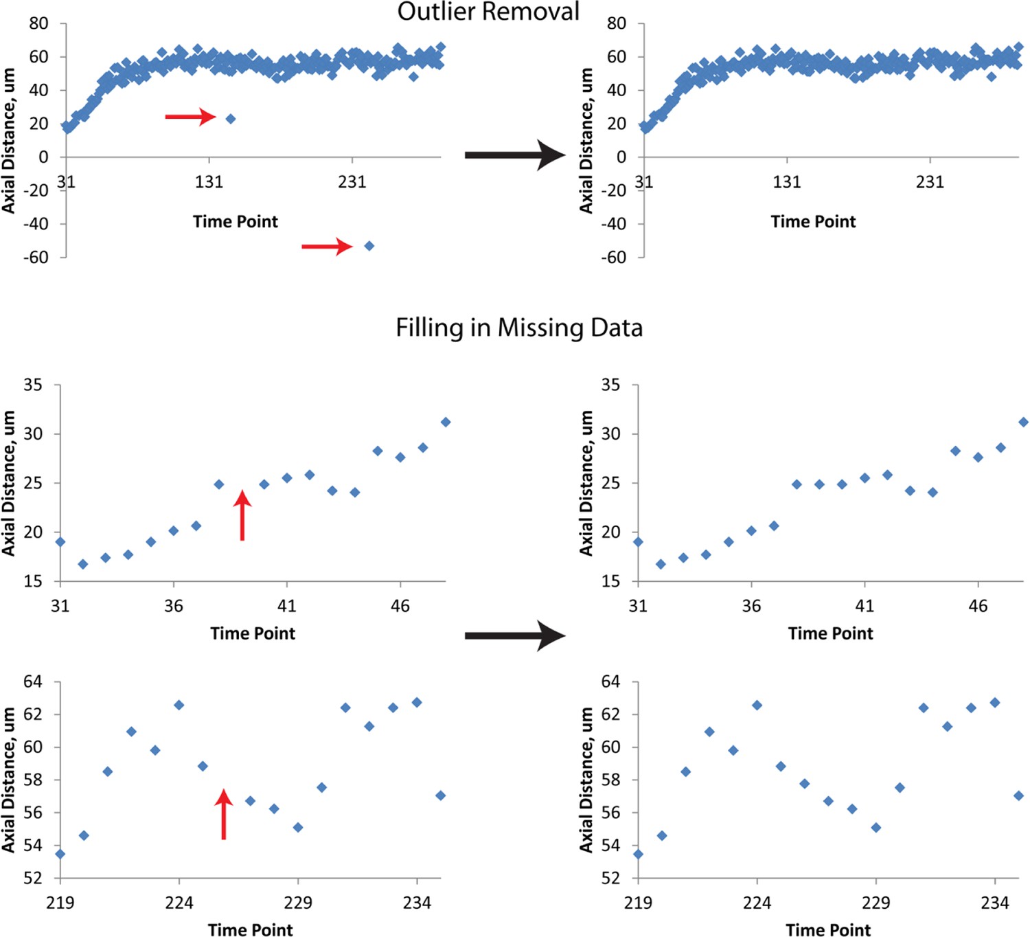
Data Post-processing.
Before fitting, raw data are treated to remove obvious outliers (top row) and to fill in missing data (mid, bottom rows). In both cases, outliers and ‘gaps’ within data are found manually, and replaced by averaging the data points immediately preceding or following the outlier or gap. Examples of raw data prior to this linear interpolation are shown at left, and examples of processed data at right. The example axial distance data shown here are derived from seam cell 3. Red arrows indicate outliers or gaps. Data shown are from the left H2 seam cell nucleus.
Figure 4 with 4 supplements
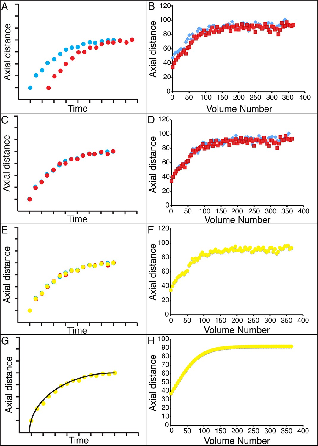
Alignment of data from different embryos.
(A,B) Axial seam cell nuclear trajectories from different embryos are similar in shape, but shifted in time. (C,D) Shifting in time aligns the trajectories. (E, F) Averaging the shifted trajectories. (G, H) Fitting the shifted trajectories. Left graphs: cartoon schematic, Right graphs: data. For clarity, we have shown the shifting, averaging, and fitting process for two embryos, but note that to construct our 'composite' model of seam cell nucleus behavior we have applied the same process to five embryos (see 'Materials and methods' for further details).
Figure 4—figure supplement 1
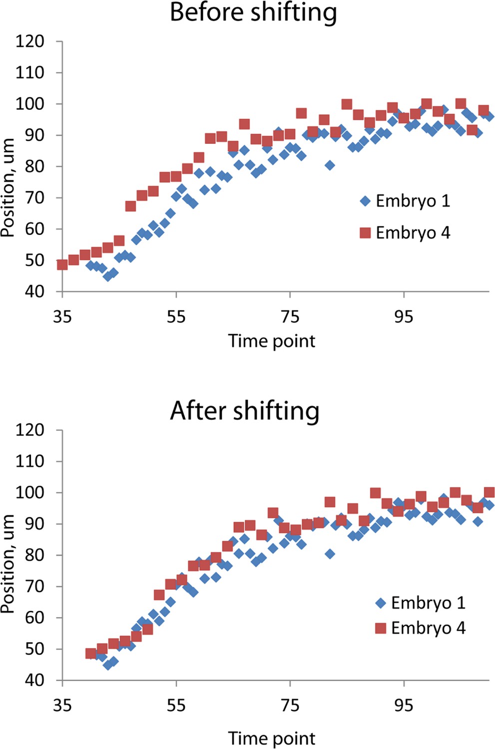
Temporal alignment of embryo data.
Data from two embryos are shown before (top) and after (bottom) temporal alignment. The data derived from embryo 4 was shifted 5 timepoints to the right, following the procedure described in 'Materials and methods'. Data shown are the z positions from the right V3 seam cell nucleus. Only a portion of the data, at early timepoints, is shown to highlight the shifting procedure.
Figure 4—figure supplement 2
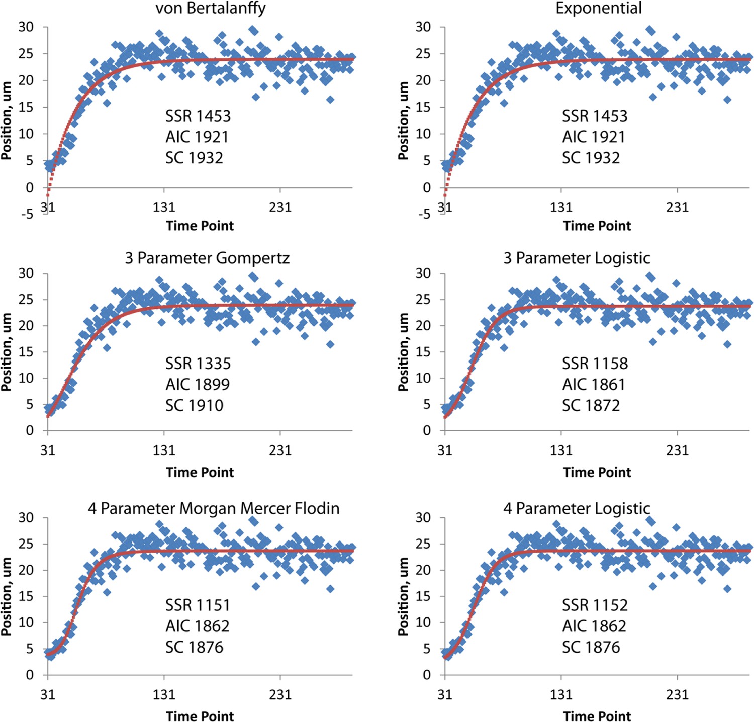
Different fits for axial displacement.
Different fitting models (see also Table 2) for embryonic axial displacement are plotted (red curves), against raw data (blue diamonds). Also shown on each plot are quantitative measures of goodness of fit: the squared sum of residuals (SSR), the Akaike Information Criterion (AIC), and the Schwarz Criterion (SC). Of the three-parameter fits, the three-parameter logistic provides the best overall fit, both from visual inspection and quantitatively (lowest SSR, AIC, and SC scores). The four-parameter Morgan Mercer Flodin and Logistic curves show slightly better qualitative fits, especially at early time points, but require careful tuning of the initial parameters to converge. For all axial displacement data shown elsewhere in the paper, the three-parameter logistic curve was used as a fitting function. Although the axial displacement data shown here are derived from the left seam cell nucleus H0, we observed the same trends for all seam cells.
Figure 4—figure supplement 3
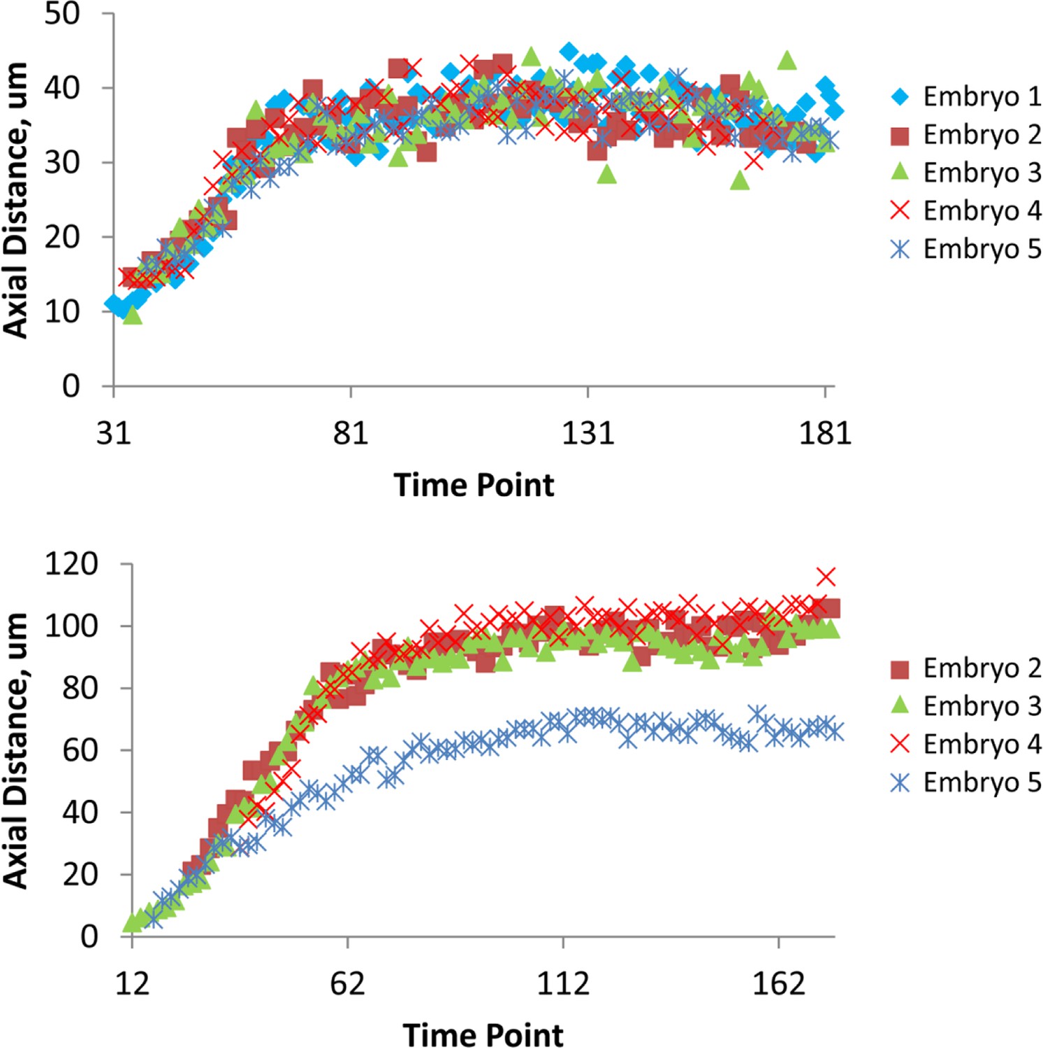
Variability in axial distance amongst different embryos.
Comparisons in axial position vs. time for a seam cell nucleus (right H1, upper graph) and for CANL (lower graph). For most nuclei, as in the upper graph, positions were stereotyped to within 4.6 μm (as quantified by <<σZ>time>seam cell; see also 'Materials and methods'). As indicated in the lower graph, we noticed CANs in embryo 5 traveled a shorter distance than in other embryo datasets (resulting in a larger value of <σZ>time for CANL, see Supplementary file 2). Data are shown after applying the shifting procedure described in 'Materials and methods'.
Figure 4—figure supplement 4
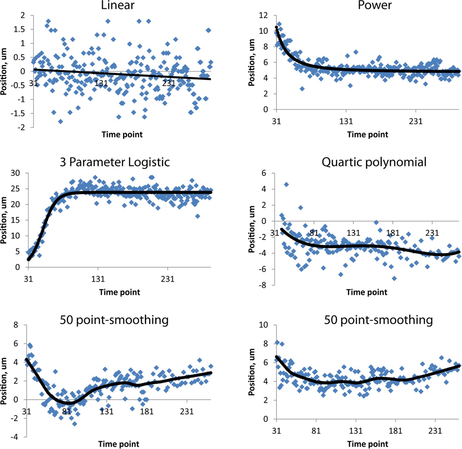
Fits used in this paper.
Examples of raw, averaged data (derived from 4 to 5 embryos, blue dots) and fits (black lines). Linear, power, and three-parameter logistic curve examples were taken from the right H0 seam cell nucleus, the quartic polynomial example from AIYL, and the smoothing fits from CANR. See also Table 1. Note the different ranges in ordinate axes.
Figure 5 with 1 supplement
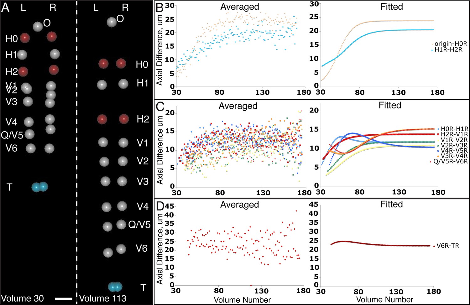
Variability in seam cell nucleus axial movement in the elongating embryo.
(A) Snapshots of the elongating embryo near start (Volume 30, left) and end (Volume 113) of elongation. Seam cell nuclei volumes are indicated as filled spheres, L/R axes are as indicated, seam cell nuclear identities indicated at the side of each snapshot, as is the origin (nose, ‘O’). See also Videos 3,4. Scalebar: 10 μm. (B–D) Axial differences over the course of elongation between adjacent seam cell nucleus pairs, sorted into greatest (B), intermediate (C), and least (D) bins, corresponding to red, gray, and blue coloring indicated in (A). Left graphs: raw, averaged data (as in Figure 4E, 4F). Right graphs: fitted data (as in Figure 4G, 4H).
Figure 5—figure supplement 1
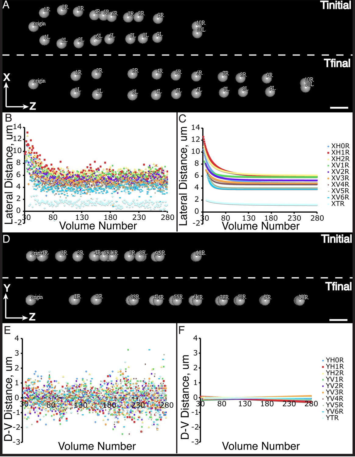
Seam cell nucleus XY movement in the elongating embryo.
(A–D) Snapshots of the elongating embryo at start (above dashed line) and end (below dashed line) of elongation, as shown in lateral (X motion, A) and dorsal-ventral (Y motion, C) views. Distances from the origin in X (B, C) and Y (E,F) are also shown for each seam cell nucleus. Both averaged (B, E) and fitted (C, F) distances are displayed. Scalebars: 10 μm.
Figure 6 with 2 supplements
Neurons and neurites in the developing embryo.
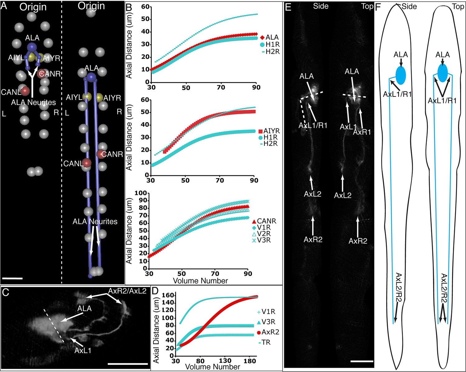
(A) Early (left) and late (snapshots) in the elongating embryo. Gray spheres: seam cell nuclei; ALA cell body: blue sphere; ALA neurites: blue lines; AIY cell bodies: yellow spheres; CAN cell bodies: red spheres. Compare to Videos 5,6. (B) ALA (top), AIYR (middle), and CANR (bottom) axial trajectories (red curves) in relation to neighboring seam cells (blue curves). ALA and AIY cells maintain their relative position with respect to the rest of the elongating body, while CANs migrate faster than neighboring seam cells. (C) ALA cell body and neurite in the twisted embryo, highlighting morphological features (ALA: ALA cell body; AxL1/R1: junction between ventral and posterior neurite extension; AxL2/R2: posterior tip of the ALA neurites). (D) Axial trajectory of ALA neurite tip in relation to indicated seam cells. (E) Top and side models of ALA in untwisted reference frame, indicating neurite bend and terminus. Compare to Figure 6—figure supplement 2.
Figure 6—figure supplement 1
Shifting, averaging and fitting procedures for modeling the ALA neurite.
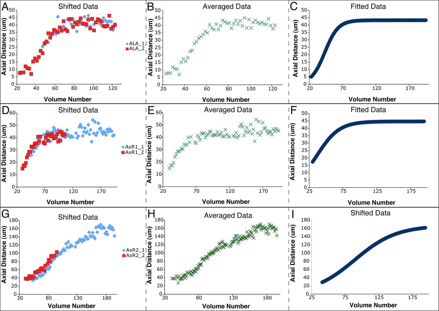
(A) Axial distance (measured from the origin point) of the ALA cell body for two ALA datasets. Similar to seam cells, axial distance increases during elongation and then plateaus once elongation has finished. (B) ALA axial distance, derived from averaging the axial distances of the shifted ALA datasets. (C) A fitted curve describing axial motion of ALA, after averaging in (B). (D–F) Shifting, averaging, and fitting of axial motion for the AxR1 point in the ALA neurite (the position at which the ventral growth of the neurite changes to posterior growth). As there is little axial growth in this part of the neurite, axial movement mirrors that of the ALA cell body. (G–I) Shifting, averaging, and fitting of axial motion for AxR2, the tip of the posteriorly-growing ALA neurite. The posterior-ward axial extension of the neurite leads to a different pattern of axial movement than for the R1 point or the ALA cell body.
Figure 6—figure supplement 2
Segmentation of neurons and neurites in the untwisted embryo.
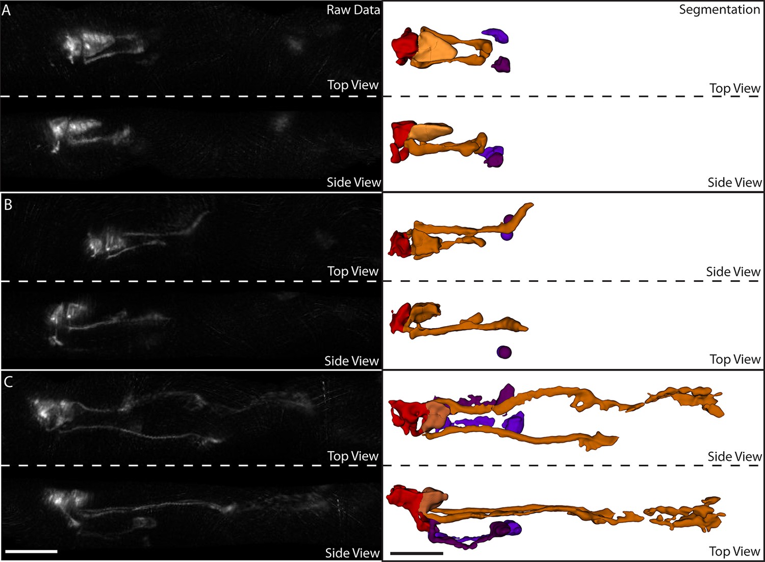
(A) Exemplary data for a twofold embryo. Left column: raw data. Right column: segmented data. The red neuron is RMED, the orange neuron is ALA, and the purple neurons are the cell bodies of the AIY neurons. At this point in embryonic development, the ALA neurites have extended ventrally and begun extending posteriorly, but have not undergone much extension. (B) Same embryo and color-scheme as in (A), but now early threefold stage. More ALA neurite extension is evident. (C) Same as in (B), but at a later stage. The ALA neurites have extended approximately 1/3 of the way to the tail at this point. In addition, neurite extension can also be observed in the AIY and RMED neurons. Scalebar: 10 μm.
Appendix 1—figure 1
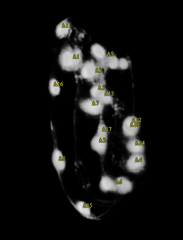
Output of the automatic seam cell nucleus detection algorithm shown before editing starts.
The markers are yellow, indicating that fewer than 20 seam cell nuclei have been labeled.
Appendix 1—figure 2
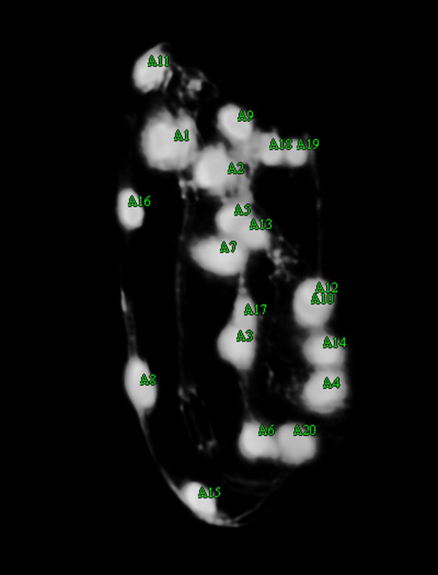
User editing.
The user shifts seam cell nucleus #9 over, adds markers for both of the 10th seam cell nuclei, shifts nucleus #6 over and adds nucleus #20. There are now 20 seam cell nuclei marked, as indicated by the green color.
Appendix 1—figure 3
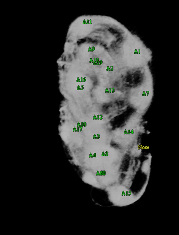
Nose labeling.
The user has increased the opacity of the volume to better enhance the appearance of the nose, now labeled in yellow.
Appendix 1—figure 4

Pairing quality control.
A potential pair is found, with the mid-point marked in red. A third seam cell nucleus is found closer to the mid-point than the pair, invalidating the pair.
Appendix 1—figure 5

Automatic lattice-building output.
The correct lattice is listed first as it had the highest rank.
Appendix 1—figure 6
The lattice after editing by the user.
https://doi.org/10.7554/eLife.10070.044
Appendix 1—figure 7
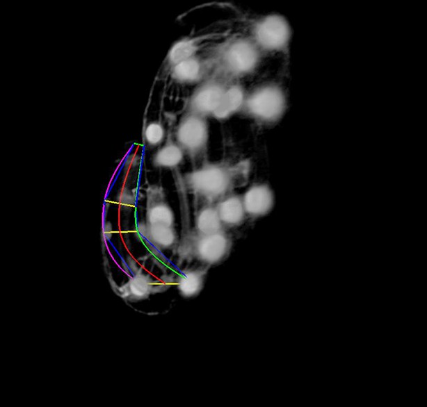
The user has started building the lattice starting at the head of the worm.
https://doi.org/10.7554/eLife.10070.045
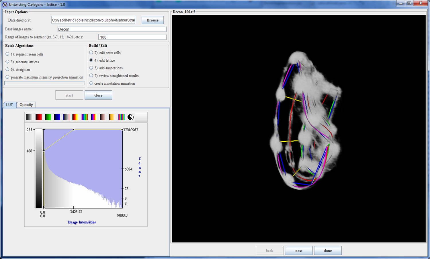
Appendix 1—figure 8
More points are added to the lattice.
The user rotates the volume to get a better view during this phase. The magenta, red, and green curves represent the left- hand curve, center-line curve, and right-hand curves respectively. The curves are natural splines which are guaranteed to pass through the user-selected lattice points while minimizing bending to produce a smooth curve that matches the shape of the worm fairly accurately.
Appendix 1—figure 9
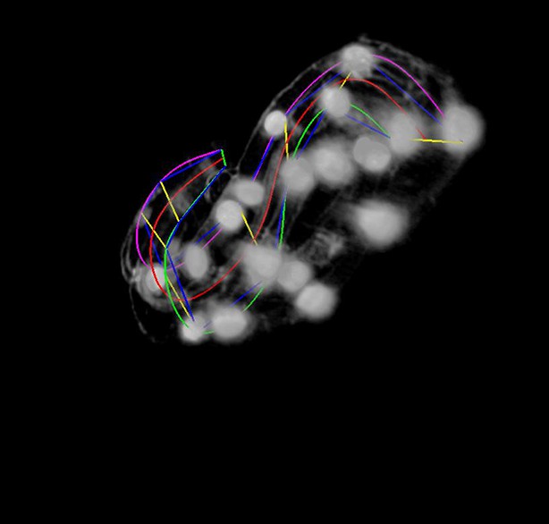
The final lattice.
Each of the 10 seam-cell pairs is marked, and 8 additional pairs have been added to capture the curve of the worm.
Appendix 1—figure 10
Annotations added to the worm volume labeling parts of the neuron.
https://doi.org/10.7554/eLife.10070.048
Appendix 1—figure 11
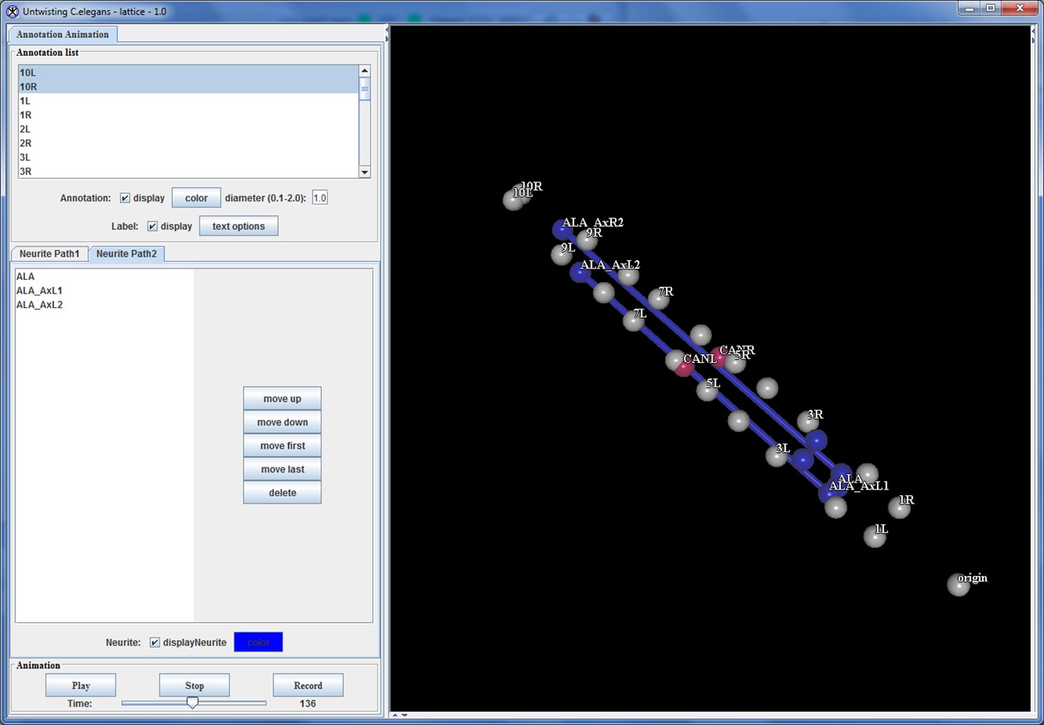
Annotation visualization tool displays changes in positions over time.
https://doi.org/10.7554/eLife.10070.049
Appendix 1—figure 12
The initial ellipse-based model of the worm.
The ellipses fit within the boundaries of the natural spline curves.
Appendix 1—figure 13
The expanded worm model.
The original ellipses are expanded until they contact an adjacent surface of the worm or they reach the boundary of the sample plane.
Appendix 1—figure 14
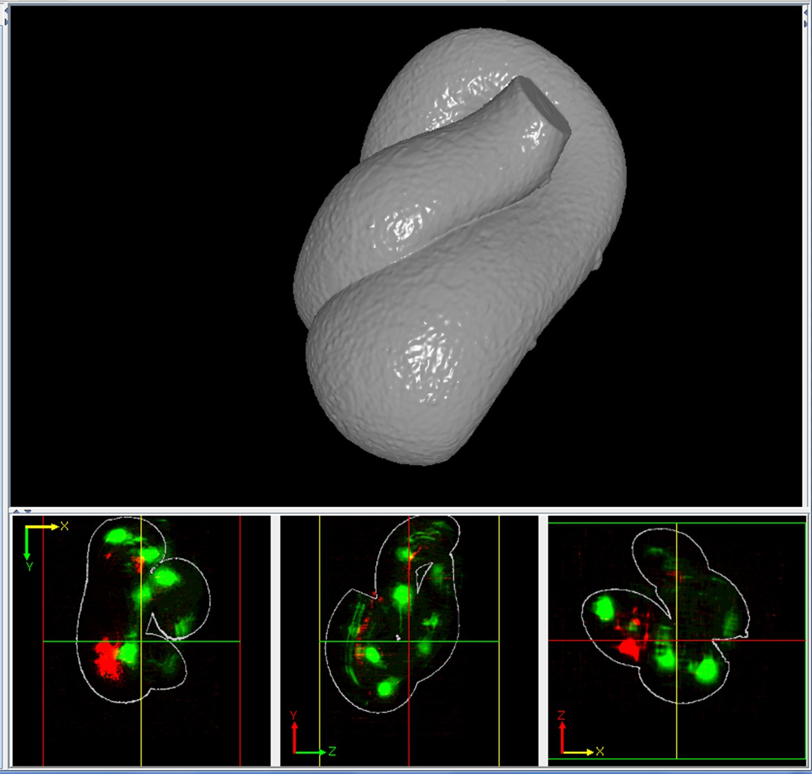
A solid representation of the worm surface.
The outlines in the bottom three panels show how the surface encapsulates the volume data.
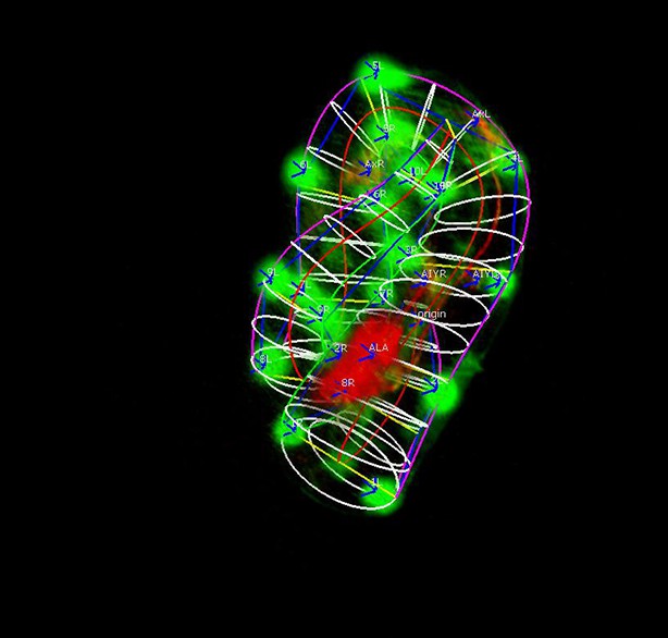
Appendix 1—figure 15
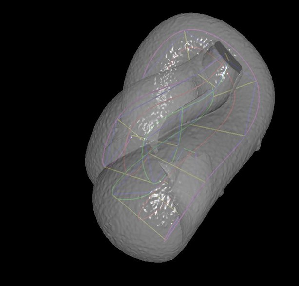
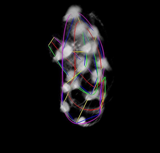
A semi-transparent view of the worm surface model, with the lattice shown inside.
https://doi.org/10.7554/eLife.10070.053
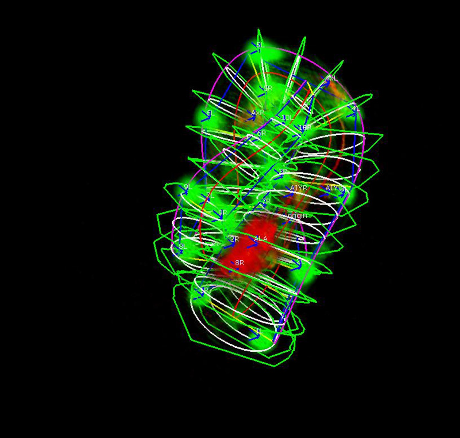
Appendix 1—figure 16
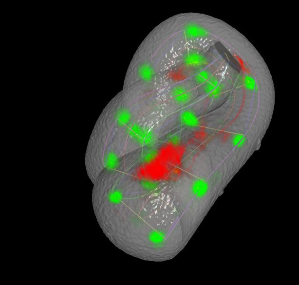
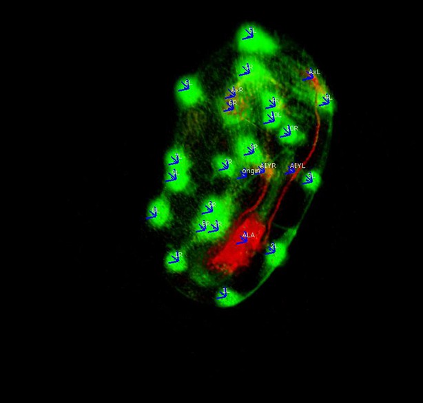
A semi-transparent view of the worm surface model displaying lattice curves, fluorescently- labeled seam cell nuclei, and neuron.
https://doi.org/10.7554/eLife.10070.054
Appendix 1—figure 17
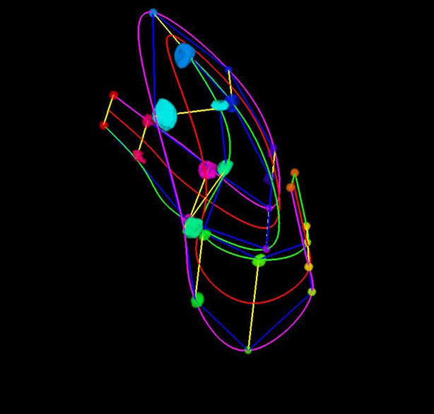
Labeled fluorescent markers.
Each pair has a unique color value, indicating which pairs belong on the same slice in the final straightened image. Labeling the lattice pairs this way helps disambiguate voxels with potential conflicts.
Appendix 1—figure 18
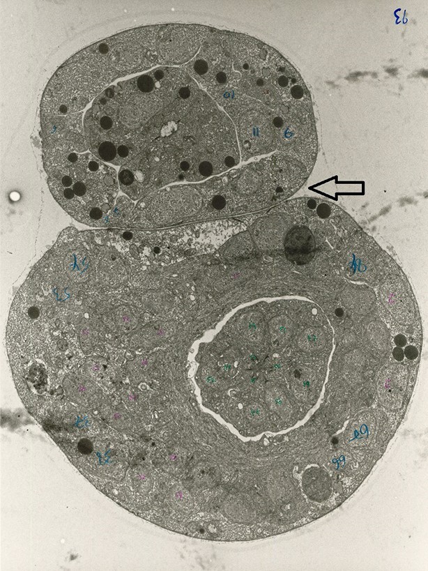
An EM image of the worm shows the worm body is flattened where overlapping segments come into contact.
https://doi.org/10.7554/eLife.10070.056Videos
Video 1
Sequential steps used in the automated lattice-building plugin.
This animation provides a graphical representation of the computational steps used to segment seam cells, build a lattice, and straighten embryo volumes. For additional information refer to Supplementary file 1 and Appendix.
Video 2
Raw data showing an untwisted worm developing from the 1.5-fold stage until hatching.
Despite errors in individual untwisted volumes, the overall pattern of embryonic development and elongation is clear.
Video 3
Rendering of seam cell nuclear positions (gray spheres) in the developing embryo viewed dorsally, from the late 1.5-fold stage until hatching.
The positions shown in the rendering are averaged, fitted values derived from five embryos, using the averaging and fitting procedure described in the text; the rendering thus represents a composite, 'best-guess' view as to seam cell evolution in a developing embryo. Times are indicated relative to the first fitted volume, and are 2.5 min apart.
Video 4
The same data as in Video 2, rendered from a side view.
https://doi.org/10.7554/eLife.10070.024
Video 5
Rendering of neurons and neurites, in the context of seam cell nuclei shown in Videos 2,3.
As in these videos, all positions are averaged, fitted values derived from multiple embryos. View is from dorsal perspective. Red spheres represent CAN cell bodies, yellow spheres represent AIY cell bodies, and blue spheres and lines correspond to ALA and its neurites. ALA and AIY cell bodies appear to closely track neighboring seam cells during elongation, while the CAN neurons actively migrate. ALA neurite outgrowth starts toward the end of elongation and continues after most other morphological changes have ceased. Times are indicated relative to the first fitted volume, and are 2.5 min apart.
Video 6
The same data as in Video 4, rendered from the side.
https://doi.org/10.7554/eLife.10070.028
Video 7
Rotating view of an untwisted L2 worm.
The image was imported into ImageJ and the Magenta LUT was applied to the stack. The volume shown here corresponds to the untwisted volume in Figure 1—figure supplement 4.
Video 8
Rotating three-dimensional view of the segmentation shown in Figure 6—figure supplement 2.
The volume was segmented and rendered in Imaris.
Tables
Table 1
Fitting functions tested for describing axial displacement. Equations are used in Figure 4—figure supplement 2. L: length; t: time. Other parameters and their meaning are listed in the table. For all axial coordinates in this paper, a three-parameter logistic function was used.
| Fitting type | Equation | Parameters |
|---|---|---|
| von Bertalanffy | L = A(1-exp[-B(t-C)]) | A: upper asymptotic length B: growth rate C: time at which L = 0 |
| Exponential | L = A-(A-B)exp(-Ct) | A: upper asymptotic length B: lower asymptotic length C: growth rate |
| Three-parameter Gompertz | L = A[exp(-exp(-B(t-C)))] | A: upper asymptotic length B: growth rate C: time at which L = 0 |
| Three-parameter logistic | L = A/[1+exp(-B(t-C))] | A: upper asymptotic length B: growth rate C: inflection point |
| Four-parameter Morgan Mercer Flodin | L = A – (A-B)/(1+(Ct)D) | A: upper asymptotic length B: length at t = 0 C: growth rate D: inflection parameter |
| Four-parameter logistic | L = B + (A-B)/{1+exp[(C-t)/D]} | A: upper asymptotic length B: lower asymptotic length C: growth rate D: steepness parameter |
Table 2
Fitting functions for each cell type. X, Y, Z trajectories were fitted as indicated functions of time (t).’ 50-point smoothing’ refers to smoothing the input data with a 50-point span, using weighted linear least squares and linear fitting.
| Cell type | X fit | Y fit | Z fit |
|---|---|---|---|
| Seam cell nucleus | Power X = atb+c | Linear Y = p1*t + p2 | Three-parameter logistic Z = A/(1+exp(-B(t-C))) |
| CANR/L | 50-point smoothing | 50-point smoothing | Three-parameter logistic Z = A/(1+exp(-B(t-C))) |
| AIYR/L | 4th degree polynomial X = p4*t4+p3*t3+p2*t2+p1*t+p0 | Linear Y = p1*t + p2 | Three-parameter logistic Z = A/(1+exp(-B(t-C))) |
| ALA ALA xR1/xL1 ALA xR2/xL2 | Linear X = p1*t + p2 | Linear Y = p1*t + p2 | Three-parameter logistic Z = A/(1+exp(-B(t-C))) |
Additional files
-
Supplementary file 1
Tutorial for use of the WormUntwisting automated lattice-building plugin.
- https://doi.org/10.7554/eLife.10070.034
-
Supplementary file 2
Deviations between embryo datasets.
For each cell studied in this paper, data from 5 embryos were shifted as discussed in the text, and the standard deviations between embryo positions at each timepoint computed. Mean standard deviations (<σ>) and the maximum standard deviation (Max(σ)) over all timepoints are recorded above. For x and y coordinates, the majority of embryo positions are within 2 μm. For z coordinates, most embryo positions lie within 10 μm of each other, with the exception of CANL. See also Figure 4—figure supplement 3 for representative embryo trajectories. For most data displayed here, at least three embryo datasets were used in generating these values. For three datasets (red italics), only two embryo datasets were compared.
- https://doi.org/10.7554/eLife.10070.035
-
Supplementary file 3
Deviations between fits and averaged data.
For each cell studied in this paper, the absolute differences between averaged coordinates and fits were computed at each time point. The means and standard deviations of these differences over time, in μm, are recorded in the table above. For x and y coordinates, the majority of fitted points lie within 1.5 μm of the averaged data, regardless of cell type. For z coordinates, the majority of fitted points lie within 7.5 μm of the averaged data, with the exception of CANL.
- https://doi.org/10.7554/eLife.10070.036
-
Supplementary file 4
Raw annotation data for seam cell nuclei, neuronal cell bodies, and ALA neurites.
Supplementary data file 4 contains raw annotation data generated by the untwisting algorithm for the 20 seam cell nuclei; CAN, AIY, and ALA cell bodies; and ALA neurites. Each sheet contains positional information for one cell, broken up by embryo dataset. Embryo datasets are labeled in the form Embryo_#_X_minutes, where # corresponds to the number assigned to the dataset (1–8) and X represents the imaging frequency (between volumes) in minutes. For each embryo dataset, the volume numbers and X, Y, and Z-positions of the cell or neurite in that volume are listed.
The data are provided in raw form, after sorting by embryo, cell, and volume but before cleaning, shifting, and fitting. For some volumes annotation information was not captured, usually due to errors in the untwisting process; for these volumes the spreadsheet entries are left blank. Additionally, there is unconstrained rotation around the midline in most datasets, which can cause X and Y-values to switch between positive and negative sign. The canonical orientation of the embryo for this paper is for cells on the right side (R) of the animal to have positive X-values and Y-positions located dorsal to the midline to have positive values; in volumes where the XR values are negative the sign should be changed, as well as the corresponding sign for the YR, XL, and YL values for that volume. Z-measurements are insensitive to this rotation. All annotations are in μm.
- https://doi.org/10.7554/eLife.10070.037
-
Supplementary file 5
Quality control measurements.
The data provided in this supplementary data file correspond to the quality control measurements used to generate Figure 2 and Figure 2—figure supplement 1. The data are sorted by embryo, volume, and measurement type. Embryos are named in the form Embryo_#_X_minutes, where # corresponds to the number assigned to the dataset (1–8) and X represents the imaging frequency (between volumes) in the dataset. All data are listed in μm.
- https://doi.org/10.7554/eLife.10070.038
Download links
A two-part list of links to download the article, or parts of the article, in various formats.
Downloads (link to download the article as PDF)
Open citations (links to open the citations from this article in various online reference manager services)
Cite this article (links to download the citations from this article in formats compatible with various reference manager tools)
Untwisting the Caenorhabditis elegans embryo
eLife 4:e10070.
https://doi.org/10.7554/eLife.10070


