Figures and data in A differentiable Gillespie algorithm for simulating chemical kinetics, parameter estimation, and designing synthetic biological circuits | eLife

Figures
Additional files

10 figures and 1 additional file

Figures

Figure 1

Download asset Open asset

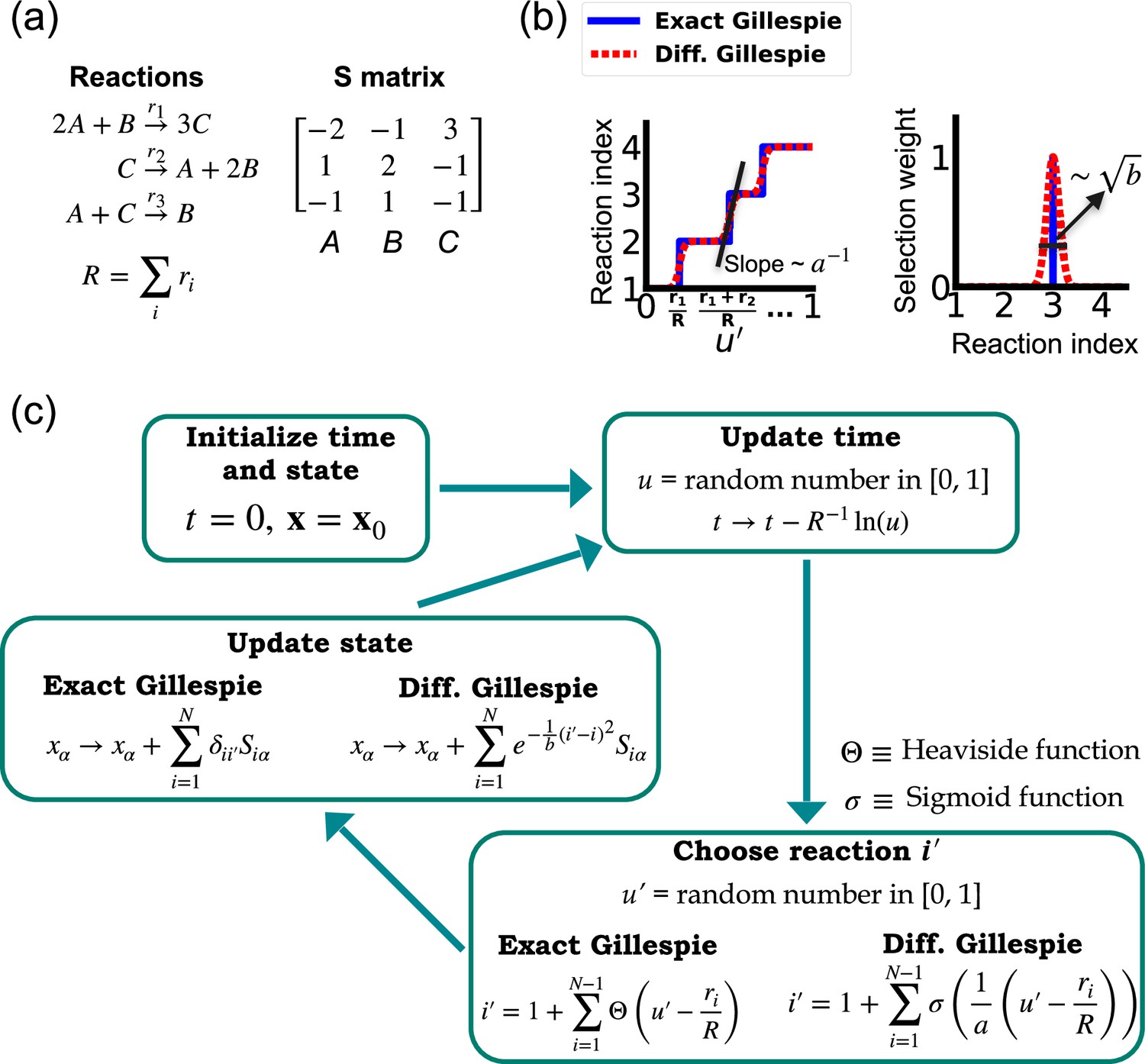
Comparison between the exact Gillespie algorithm and the differentiable Gillespie algorithm (DGA) for simulating chemical kinetics.

(a) Example of kinetics with $N = 3$ reactions with rates $r_{i} (i = 1, 2, 3)$ . (b) Illustration of the DGA’s approximations: replacing the non-differentiable Heaviside and Kronecker delta functions with smooth sigmoid and Gaussian functions, respectively. (c) Flow chart comparing exact and differentiable Gillespie simulations.

Figure 2

Download asset Open asset

Flow chart of the parameter optimization process using the differentiable Gillespie algorithm (DGA).

The process begins by initializing the parameters $\vec{θ} = \vec{θ_{0}}$ . Simulations are then run using the DGA to obtain statistics ${S_{i} (\vec{θ})}$ like moments. These statistics are used to compute the loss $L ({S_{i}})$ , and the gradient of the loss $\nabla L$ is obtained. Finally, parameters are updated using the ADAM optimizer, and the process iterates to minimize the loss.

Figure 3

Download asset Open asset

Two-state gene regulation architecture.

(a) Schematic of gene regulatory circuit for transcriptional repression. RNA polymerase (RNAP) binds to the promoter region to initiate transcription at a rate $r$ , leading to the synthesis of mRNA molecules (red curvy lines). mRNA is degraded at a rate $γ$ . A repressor protein can bind to the operator site, with association and dissociation rates $k_{on}^{R}$ and $k_{off}^{R}$ , respectively. (b) Experimental data from Phillips et al., 2019, showing the relationship between the mean mRNA level and the Fano factor for two different promoter constructs: lacUD5 (green squares) and 5DL1 (red squares).

Figure 4

Download asset Open asset

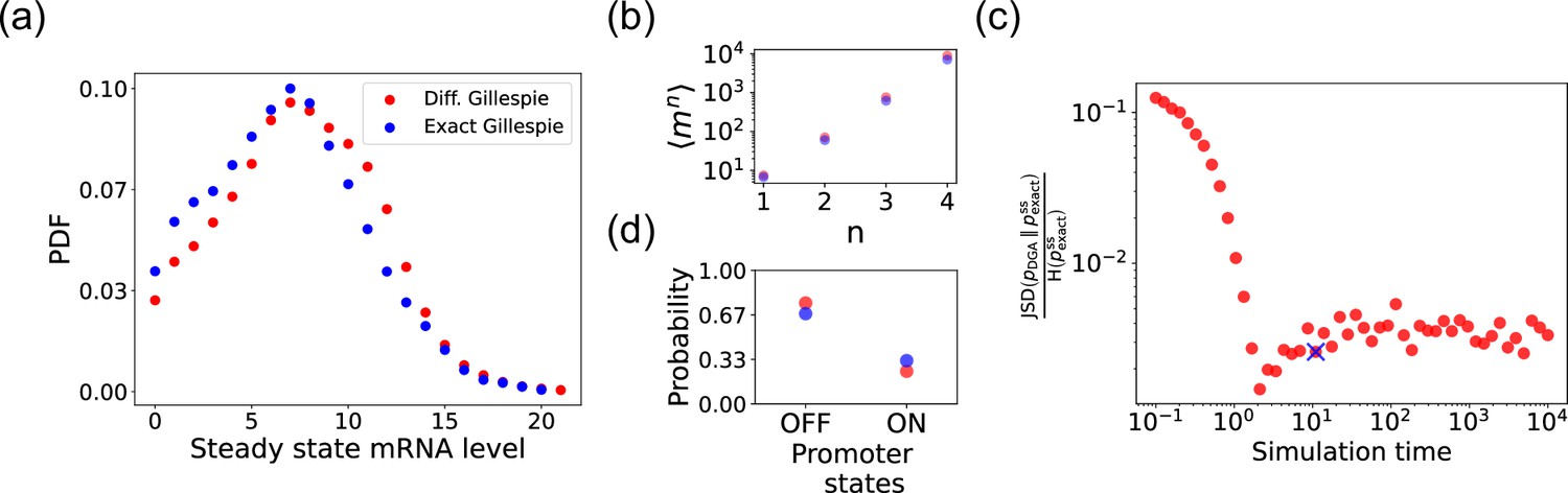
Accuracy of the differentiable Gillespie algorithm (DGA) in simulating the two-state promoter architecture in Figure 3a.

Comparison between the DGA and exact simulations for (a) steady-state mRNA distribution, (b) moments of the steady-state mRNA distribution, and (d) the probability for the promoter to be in the ‘ON’ or ‘OFF’ state. (c) Ratio of the Jensen–Shannon divergence $JSD (p_{DGA} | | p_{exact}^{ss})$ between the differentiable Gillespie probability distribution function (PDF) $p_{DGA}$ and the exact steady-state PDF $p_{exact}^{ss}$ , and the Shannon entropy $H (p_{exact}^{ss})$ of the exact steady-state PDF. In all of the plots, 2000 trajectories are used. The simulation time used in panels (a), (b), and (d) is marked by blue ‘x’. Parameter values: $k_{on}^{R} = 0.5$ , $k_{off}^{R} = 1.0$ , $r = 10$ , $γ = 1$ , $1 / a = 200$ , and $1 / b = 20$ .

Figure 5

Download asset Open asset

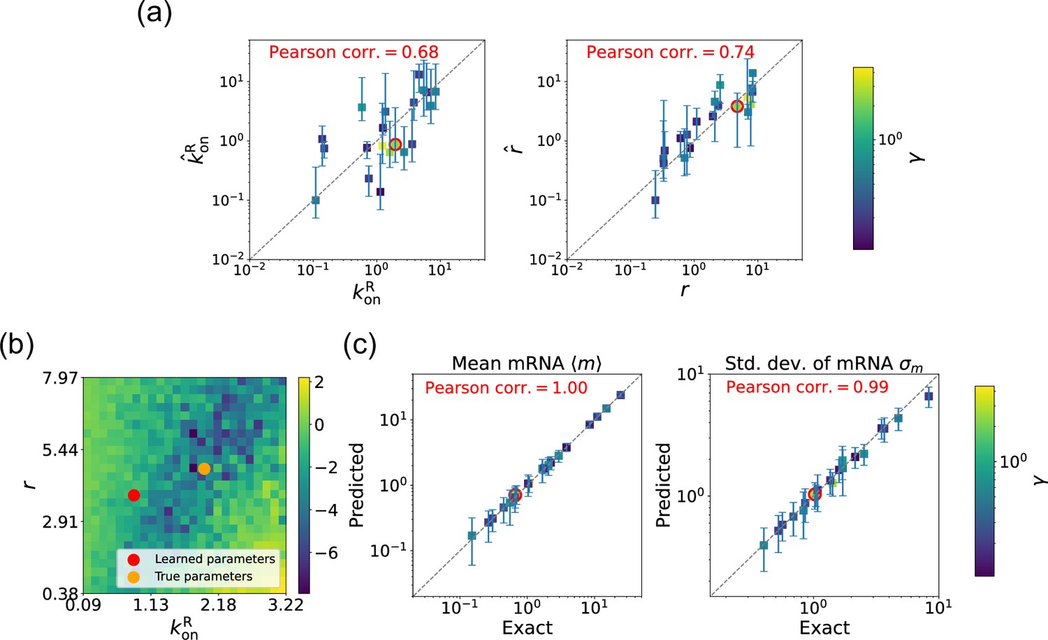
Gradient-based learning via differentiable Gillespie algorithm (DGA) is applied to the synthetic data for the gene expression model in Figure 3a.

Parameters $k_{off}^{R}$ are fixed at 1, with $1 / a = 200$ and $1 / b = 20$ for a simulation time of 10. (a) Scatter plot of true versus inferred parameters ( ${\hat{k}}_{on}^{R}$ and $\hat{r}$ ) with $γ$ constant. Error bars are 95% confidence intervals (CIs). Panel (b) plots the logarithm of the loss function near a learned parameter set (shown in red circles in (a)), showing insensitivity regions. Panel (c) compares true and predicted mRNA mean and standard deviation with 95% CIs.

Figure 6

Download asset Open asset

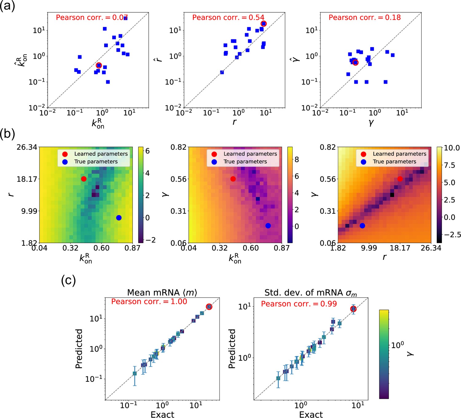
Gradient-based learning via differentiable Gillespie algorithm (DGA) is applied to the synthetic data for the gene expression model in Figure 3a.

Parameters $k_{off}^{R}$ are fixed at 1, with $1 / a = 200$ and $1 / b = 20$ for a simulation time of 10. (a) Scatter plot of true versus inferred parameters ( ${\hat{k}}_{on}^{R}$ , $\hat{r}$ , and $γ$ ). Error bars are 95% confidence intervals (CIs). Panel (b) plots the logarithm of the loss function near a learned parameter set (shown in red circles in (a)), showing insensitivity regions. Panel (c) compares true and predicted mRNA mean and standard deviation with 95% CIs.

Figure 7

Download asset Open asset

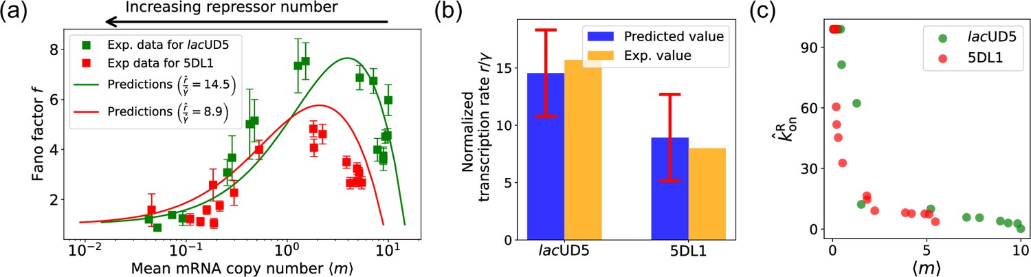
Fitting of experimental data from Jones et al., 2014 using the differentiable Gillespie algorithm (DGA).

(a) Comparison between theoretical predictions from the DGA (solid curves) and experimental values of mean and the Fano factor for the steady-state mRNA levels are represented by square markers, along with the error bars, for two different promoters, lacUD5 and 5DL1. Solid curves are generated by using DGA to estimate $\hat{r}$ , $\hat{γ}$ , and ${{\hat{k}}_{on}^{R}}$ and using this as input to exact analytical formulas. (b) Comparison between the inferred values of $\frac{\hat{r}}{\hat{γ}}$ using DGA with experimentally measured values of this parameter from Jones et al., 2014. (c) Inferred ${\hat{k}}_{on}^{R}$ values as a function of the mean mRNA level.

Figure 8

Download asset Open asset

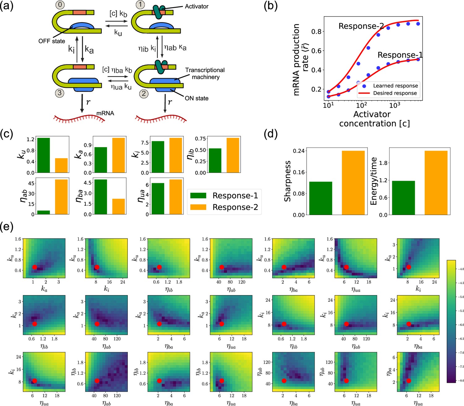
Design of the four-state promoter architecture using the differentiable Gillespie algorithm (DGA).

(a) Schematic of four-state promoter model. (b) Target input–output relationships (solid curves) and learned input–output relationships (blue dots) between activator concentration $[c]$ and average mRNA production rate. (c) Parameters learned by DGA for the two responses in (b). (d) The sharpness of the response $\frac{d ⟨ \bar{r} ⟩}{d [c]} [c]$ , and the energy dissipated per unit time for two responses in (b). (e) Logarithm of the loss function for the learned parameter set for Response-2, revealing directions (or curves) of insensitivity in the model’s parameter space. The red circles are the learned parameter values.

Appendix 1—figure 1

Download asset Open asset

In panels (a) and (b), we plot the ratio of the Jensen–Shannon divergence $JSD (p_{DGA} | | p_{exact}^{ss})$ between the differentiable Gillespie PDF $p_{DGA}$ and the exact steady-state PDF $p_{exact}^{ss}$ , and the Shannon entropy $H (p_{exact}^{ss})$ of the exact steady-state PDF, as a function of the two sharpness parameters $1 / a$ and $1 / b$ .

In panel (a), $1 / b = 20$ ; in panel (b), $1 / a = 200$ . The simulation time is set to 10. In panels (c) and (d), for these same values, we show the gradient ${\nabla L}_{r}$ of the loss function $L$ with respect to the parameter $r$ near the true parameter values. In all the plots, the values of the rates are: $k_{on}^{R} = 0.5$ , $k_{off}^{R} = 1$ , $r = 10$ , and $γ = 1$ . 5000 trajectories are used to obtain the PDFs, while 200 trajectories are used to obtain the gradients.

Appendix 3—figure 1

Download asset Open asset

Error bars estimation for asymmetric loss function.

Additional files

MDAR checklist: https://cdn.elifesciences.org/articles/103877/elife-103877-mdarchecklist1-v1.pdf
Download elife-103877-mdarchecklist1-v1.pdf

Download links

A two-part list of links to download the article, or parts of the article, in various formats.

Downloads (link to download the article as PDF)

Article PDF

Open citations (links to open the citations from this article in various online reference manager services)

Mendeley

Cite this article (links to download the citations from this article in formats compatible with various reference manager tools)

Krishna Rijal
Pankaj Mehta

(2025)

A differentiable Gillespie algorithm for simulating chemical kinetics, parameter estimation, and designing synthetic biological circuits

eLife 14:RP103877.

https://doi.org/10.7554/eLife.103877.3

Sign up for email alerts

Privacy notice